


1. INTRODUCTION
Perennially ice-covered lakes in the McMurdo Dry Valleys, Antarctica have long been studied as novel habitats for life. Ice covers offer protection from wind-driven turbulence, and together with strong salinity gradients within the lakes, permit permanent vertical temperature stratification, the development of supersaturated gas concentrations (Wharton and others, Reference Wharton, McKay, Simmons and Parker1986; Priscu and others, Reference Priscu, Downes and McKay1996; Andersen and others, Reference Andersen, McKay and Wharton1998) and altered sediment pathways (Doran and others, Reference Doran, Wharton and Lyons1994). Although the permanent ice covers provide insulation from the atmosphere, they do allow penetration of solar radiation, often producing thermal maxima deep in the water column in association with saltier water (Vincent and others, Reference Vincent, Mueller and Vincent2008). Despite the deep temperature maxima, the salt gradient maintains vertically stable water columns (Spigel and Priscu, Reference Spigel and Priscu1996). Ice cover thickness is balanced primarily by ablation at the surface and ice growth at the bottom (Chinn, Reference Chinn, Green and Friedmann1993; Adams and others, Reference Adams, Priscu, Fritsen, Smith, Brackman and Priscu1998). McKay and others (Reference McKay, Clow, Wharton and Squyres1985) developed a steady-state energy-balance model that predicts ice cover thickness based on surface ablation (mass loss by all means) rates and latent heat of ice formation. Latent heat release, associated with ice growth, is conducted upwards and lost to the atmosphere due to ablation (McKay and others, Reference McKay, Clow, Wharton and Squyres1985). Because of the tight coupling of lake ice thickness to atmospheric processes, the ice covers should respond directly to changing climate (Wharton and others, Reference Wharton1992; Launiainen and Cheng, Reference Launiainen and Cheng1998; Reid and Crout, Reference Reid and Crout2008).
Lakes in Taylor Valley, one of the McMurdo Dry Valleys, have been perennially ice covered since at least 1903, when they were discovered by Robert Falcon Scott (Scott, Reference Scott1905). Taylor Valley lake volumes are controlled by a balance of summer temperatures high enough to generate melt from local glaciers, yet low enough for the lake ice covers to persist through the summer (Chinn, Reference Chinn, Green and Friedmann1993). The interannual variability of ice thicknesses in Taylor Valley lakes varied between 3 and 6 m over the past two decades (McKay and others, Reference McKay, Clow, Wharton and Squyres1985; Doran and others, Reference Doran2002b) and fluctuated by ~1 m during each seasonal cycle. Ice thickness of Lake Hoare (freshwater lake) in McMurdo Dry Valleys thinned from 1977 to 1986 at a rate of >0.28 m a−1 (Wharton and others, Reference Wharton, Simmons and McKay1989); however little climate data are available for this time period. Between 1986 and 1999, the lake-ice thickness increased at a rate of 0.11 m a−1 in association with an annual air temperature decrease of 0.7°C (10 a)−1 (Doran and others, Reference Doran2002b). This period of pronounced cooling was terminated by one of the warmest summers on record, resulting in a significant lake level rise (Barrett and others, Reference Barrett2008; Doran and others, Reference Doran2008). Following this warm pulse, lake-ice thicknesses have been decreasing since early- to mid-2000 at rates between 0.07 and 0.18 m a−1 (unpublished data). Here we present results from a lake ice model that allowed us to differentiate between the influence of atmospheric processes (i.e. changes in climate) and the long-term heat storage in the water column on lake ice thickness.
2. SITE DESCRIPTION
The McMurdo Dry Valleys, East Antarctica are an ice-free region with perennially ice-covered lakes typically located in hydrologically closed basins. This arid environment results from a combination of low precipitation and the Transantarctic Mountains blocking the ice-sheet flow (Chinn, Reference Chinn, Green and Friedmann1993). The mean annual valley-bottom temperatures range from −14.8°C to −30.0°C, with summer temperatures high enough to enable glacial melt, which feeds into the lakes (Doran and others, Reference Doran2002a). The two lakes in this study, west lobe of Lake Bonney (WLB) and Lake Fryxell (Fig. 1), are in different microclimatic zones in Taylor Valley. WLB is located ~27 km from the coast and influenced by strong, dry winds from the Antarctic plateau, whereas Lake Fryxell, adjacent to the coast, is influenced by moist coastal winds (Fountain and others, Reference Fountain1999; Doran and others, Reference Doran2002a). Lake levels in Taylor Valley have been rapidly increasing since the early 2000s and the depths of WLB and Lake Fryxell, as of January 2012 are 41.2 and 22.4 m, respectively.
Fig. 1. Map of Taylor Valley, Antarctica. Triangles indicate locations of meteorological stations.
3. MODEL DEVELOPMENT
3.1. General model description
Launiainen and Cheng (Reference Launiainen and Cheng1998) provide a general description and evolution of different ice models since thermodynamic modeling of ice began in the late 1800s. Despite extensive research, no universal lake ice model is available, as each lake has different characteristics and unique adjustments are necessary (Reid and Crout, Reference Reid and Crout2008). The model we have developed uses generalized parameters to make it adaptable to other stratified perennially ice-covered lakes.
The model developed here is modified from an approach by Launiainen and Cheng (Reference Launiainen and Cheng1998) and Reid and Crout (Reference Reid and Crout2008). The model considers: (1) the dynamic coupling of atmospheric processes with ice (surface energy balance), (2) the dynamic coupling of the water column with ice (moving boundary condition) and (3) heat conduction within the ice and the water column (two 1-D heat equations) (Fig. 2). Three boundaries are defined in the model: atmosphere/ice, ice/water and water/bedrock. The vertical temperature profile of the ice and the water column is solved using a spectral method based on the state of the boundaries. The heat equation in both regions, along with the interface equation, were discretized in space using the Chebyshev pseudo-spectral method (N = 16) and in time using an implicit method. The discrete system was solved using a Newton–Krylov method. The main advantage of the spectral method over the finite difference or the finite element method is a higher degree of accuracy for smooth problems allowing a coarse computational grid (Trefethen, Reference Trefethen2000).
Fig. 2. Conceptual representation of heat fluxes and temperature profile for WLB. Numbers in boxes represent annually averaged fluxes (W m−2).
Surface ice temperature was calculated based on the summation of surface radiative fluxes and becomes the top boundary condition for the 1-D heat equation (Section 3.4). Known surface ice temperature allows for the calculation of temperature profiles of the ice as the temperature at the bottom of the ice is set to the freezing point. The water temperature profile is solved using a second 1-D heat equation, with penetrating solar radiation acting as the heat flux contribution to the water column (water/bedrock boundary temperature is fixed). Ice and water temperature profiles are coupled at the ice/water interface accounting for the conductive, latent and sensible heat fluxes. The ice/water interface is a moving Dirichlet boundary condition, which forces the solution of a heat equation to converge at the freezing point of the water. This boundary incorporates latent heat fluxes associated with the phase transition (Gupta, Reference Gupta2003).
A 1-D solution to the heat equation is valid because it succinctly approximates the physical processes. The lateral thermal gradient can be considered negligible with regards to depth, allowing a 1-D heat equation to be employed because vertical exchanges are much greater than lateral exchanges. Heat exchange within the ice is assumed to occur through conduction (even though this assumption can break down when ice is isothermal) and is based on a temperature gradient defined at the atmosphere/ice and ice/water boundaries. The heat within the ice diffuses vertically at a rate defined by the thermal diffusivity of the ice and the temperature gradient. Similar to the approach used for the ice, a 1-D heat equation is used to calculate the temperature profile of the water column in order to better constrain heat fluxes at the ice/water boundary. The water column of Taylor Valley lakes we modeled are chemically stratified and vertical diffusive heat transfer occurs at the molecular level; our study lakes have no vertical convective mixing (Spigel and Priscu, Reference Spigel, Priscu and Priscu1998). Horizontal motion in the lakes can occur as the result of horizontal advection caused by lateral stirring induced by contact with glacial ice (WLB) and stream input during the austral summer (Spigel and Priscu, Reference Spigel, Priscu and Priscu1998) and are not considered in this model.
The model employs dimensional analysis permitting the grouping of variables that describe physical parameters in a dimensionless form. Dimensional analysis is based on the Buckingham π-theorem, allowing for the reduction of independent variables by k dimensions, where k represents physical dimensions required to describe n variables used in the model. Then, it follows that there will be π dimensionless groups based on n – k (Yarin, Reference Yarin2012). As a result, this method reduces the complexity of the model and, consequently, reduces the complexity of the solution to the heat equation and allows the computational domain to be fixed at [−1, 1], regardless of the ice thickness.
3.2. Model input data
Meteorological data used in the model include air temperature, shortwave radiation (400–1100 nm), relative humidity and wind speed. Longwave upwelling and downwelling radiation, and turbulent sensible and latent heat fluxes were parameterized using equations adapted from Reid and Crout (Reference Reid and Crout2008), discussed in more detail below. The albedo of the ice was simulated as a spline function based on a 5-month data record (September–February) from WLB, obtained from Fritsen and Priscu (Reference Fritsen and Priscu1999). Based on this record, the largest albedo change (increase) occurs during the summer months when ice morphology and hoar frost in air bubbles change due to the thermal properties of the ice (Adams and others, Reference Adams, Priscu, Fritsen, Smith, Brackman and Priscu1998; Fritsen and Priscu, Reference Fritsen and Priscu1999). The missing albedo data for the remainder of the year (spring and fall) were extrapolated. Any error in this assumption is reduced by the diminished importance of shortwave radiation during these periods and the complete lack of shortwave radiation during the winter months.
The model was run with 16 a of meteorological data obtained from Lake Bonney's weather station, located on the southern shore of east lobe of Lake Bonney (Fig. 1). Data were collected using Campbell Scientific dataloggers (CR10 and 21X) at 30 s sampling intervals and stored as 15 min averages (Doran and others, Reference Doran, Dana, Hastings and Wharton1995, Reference Doran2002a). Air temperature was measured using Campbell 207 and 107 temperature probes at a 3 m height (Doran and others, Reference Doran, Dana, Hastings and Wharton1995). Shortwave radiation was obtained with Li-Cor LI200S and LI200X silicon pyranometer (Doran and others, Reference Doran, Dana, Hastings and Wharton1995). Wind speed was obtained with R.M. Young model 05103 wind monitors (Doran and others, Reference Doran, Dana, Hastings and Wharton1995). The model was run at 12 h intervals, dynamically averaging high-resolution data (15 min intervals) during simulations.
Gaps in data occurred, ranging from hours to months, due to either failed sensors or failed dataloggers. Missing shortwave radiation was remedied by using well-known published equations (Section 3.5) dynamically substituting gaps in data during model simulations. Missing air temperature values were substituted by using a function based on daily averaged temperatures from 16 a of data. Missing relative humidity and wind speed data represent cumulative 6.6 and 4.6% of the entire dataset respectively, and were determined by a uniform random number generator (within the upper and lower limit of each variable). Uniform distribution ensures that a value within the set range has equal probability of being generated.
3.3. Validation data
Ice thickness data were measured manually at the drill hole sites from the bottom of the ice to the piezometric water level, representing the ice (w.e.) thickness. Due to logistical constraints, the ice thickness data were only available during the austral summers when the ice was most dynamic, with the exception of an extended season in 2008, when data were obtained through austral autumn (into March). Replicate ice thickness measurements (3–10) were made during the same day (within a 10 m2 grid) or within 2 d of each other, and show a large variability (largest standard deviation of seasonally measured ice thickness is 0.54 m), introducing error during the validation procedure of the model.
Continuous ablation data were measured from suspended pressure transducers at the bottom of the ice (Dugan and others, Reference Dugan, Obryk and Doran2013). Data were recorded at 1 min intervals (averaged over 20 min), using Druck PDCR 1830 or Keller Series 173 pressure transducers and stored on Campbell Scientific CR10X and CR1000 dataloggers (Dugan and others, Reference Dugan, Obryk and Doran2013).
3.4. Surface energy balance
The vertical temperature profile of the ice and its evolution over time can be modeled utilizing a 1-D unsteady heat equation:
 $$pc\displaystyle{{\partial T(z,t)} \over {\partial t}} = - \displaystyle{\partial \over {\partial z}}\left( { - k\displaystyle{{\partial T(z,t)} \over {\partial z}} + I(z,t)} \right)$$
where p is the density of ice or water, c is the specific heat capacity of ice or water, T is temperature, z is depth, t is time, k is thermal conductivity and I is the heat source term within the ice and the water column. All constants and variables are summarized in Appendix. Shortwave radiation is the only significant flux that contributes to the I term because ice is opaque in infrared and transparent in the visible spectrum (McKay and others, Reference McKay, Clow, Andersen and Wharton1994). The transmittance of sunlight through the perennially ice-covered lakes in Taylor Valley can be approximated using the Lambert–Beer law (McKay and others, Reference McKay, Clow, Wharton and Squyres1985), by defining a constant extinction coefficient. However, this technique does not account for the absorbed near-infrared radiation at the very surface of the ice (Brandt and Warren, Reference Brandt and Warren1993; Bintanja and van den Broeke, Reference Bintanja and van den Broeke1995). A method used in Bintanja and van den Broeke (Reference Bintanja and van den Broeke1995) was adapted that parameterized solar energy by partitioning absorbed solar energy at the very surface and subsurface of the ice, expressing the heat source term as:
 $$I(z,t) = (1 - \chi )(1 - \alpha )Q_se^{ - \kappa z}$$
where χ accounts for a fraction of absorbed shortwave radiation at the surface, α is albedo, Q s is shortwave radiation and κ is the extinction coefficient of the ice at depth z.
The top boundary condition for Eqn (1) is calculated based on the summation of all surface radiative heat fluxes:
 $$F(T_s)\, = \,\chi (1-\alpha )Q_s\, + \,Q_b\, + \,Q_d\, + \,Q_h\, + \,Q_l\, + \,F_i$$
where T s is ice surface temperature, Q s is shortwave radiation, Q b is longwave upwelling radiation, Q d is longwave downwelling radiation, Q h is sensible heat flux, Q l is latent heat flux and F i is the heat conduction at the ice surface. However, T s cannot be solved based on this equation alone because the longwave upwelling radiation, and sensible and conductive heat fluxes depend on the surface ice temperature. The Newtonian iterative method is implemented in the model to solve for T s , which is used to determine the temperature gradient within the ice cover. Positive fluxes are toward the ice, negative are away from the ice.
3.5. Shortwave radiation
Shortwave radiation (Q s ) for an atmosphere-less Earth is defined as:
 $$Q_s\, = \,ScosZ\; $$
where S is a solar constant and Z is a solar zenith, derived using solar declination, solar angle and latitude. Atmospheric attenuation of Q s requires modification of Eqn (4) with empirical parameters related to the study site and numerous equations are available in the literature (Lumb, Reference Lumb1964; Bennett, Reference Bennett1982; Reid and Crout, Reference Reid and Crout2008). Parameterization of Q s for an Antarctic site has been done by Reid and Crout (Reference Reid and Crout2008) and was adopted here.
3.6. Longwave radiation
Longwave upwelling radiation (Q b ) was modeled based on the Stefan–Boltzmann law as a function of surface ice temperature and is expressed as:
 $$Q_b\, = \, - \varepsilon _i\sigma _sT_s^4 $$
where ε i represents dimensionless surface emissivity and σ s is the Stefan–Boltzmann constant (Launiainen and Cheng, Reference Launiainen and Cheng1998).
Downwelling longwave radiation (Q d ) takes a form of Eqn (5) but is controlled by surface air temperature (T a ) and cloud cover (C) (Konig-Langlo and Augstein, Reference Konig-Langlo and Augstein1994; Guest, Reference Guest1998). Cloud cover is expressed as a unitless value (from 0 to 1) representing the fraction of sky covered by clouds. However, cloud cover data for the WLB is unavailable. Missing cloud cover data can be treated as an adjustable parameter in models driven by surface energy balance (Liston and others, Reference Liston, Winther, Brunland, Elvehoy and Sand1999). Here, we chose C to be generated by a random number generator (uniform distribution) at daily intervals in order to simplify the model by decreasing the number of adjustable parameters. Downwelling longwave radiation requires parameterization of atmospheric emissivity (ε a ), which accounts for C, vapor distribution and temperature (Konig-Langlo and Augstein, Reference Konig-Langlo and Augstein1994). The equation for Q d was adopted from Konig-Langlo and Augstein (Reference Konig-Langlo and Augstein1994) because they parameterized ε a based on Antarctic datasets, which is applicable for high latitudes:
 $$Q_d\, = \,(0.765{\rm} + {\rm} 0.22C^3)\sigma _sT_a^4 $$
3.7. Sensible and latent heat flux at the ice surface
Turbulent sensible (Q h ) and latent (Q l ) heat fluxes at the atmosphere/ice boundary are modeled after Launiainen and Cheng (Reference Launiainen and Cheng1998) and are expressed as:
 $$Q_h\, = \,\rho _ac_aC_H(\Delta T)V$$
 $$Q_l\, = \,\rho _aR_lC_E(\Delta q)V$$
where ρ a is air density, c a is specific heat capacity of air, V is wind speed, R is enthalpy of vaporization (or sublimation if T s < 273.15), ΔT is the temperature difference between the atmosphere and the ice surface, Δq is specific humidity difference between the atmosphere and the ice surface, and C H and C E are dimensionless bulk transfer coefficients. Strictly speaking, C H and C E depend on atmospheric stability (Launiainen and Cheng, Reference Launiainen and Cheng1998); however, here they are treated as constants approximated based on Parkinson and Washington (Reference Parkinson and Washington1979).
3.8. Conductive heat flux
Conductive heat flux at the surface of the ice is defined as a temperature gradient between the air and the top layer of the ice:
 $$F_i\, = \, - k\left( {\displaystyle{{\partial T} \over {\partial Z}}} \right)$$
where T represents the temperature difference defined by the depth Z, and k is the thermal conductivity of the ice. Similarly, heat conduction between ice and the water takes the form of Eqn (9).
3.9. Ice ablation and growth
Ice removal from the top of the ice is approximated as a function of net surface radiative heat fluxes, similar to Eqn (3). If the net radiative heat flux (Q net ) > 0, the excess energy is used to remove the surface layer of the ice, and can be expressed as:
 $$\displaystyle{{d_{ABL}} \over {dt}} = \; - \left( {\displaystyle{1 \over {L\rho}}} \right)Q_{net}$$
where L is latent heat of freezing and ρ is ice density. Such an approach does not distinguish between sublimation and ice melt; however, it sufficiently represents cumulative annual ice removal from the surface of the ice (Fig. 3).
Fig. 3. Linear fit between 6 a of overlapping measured and predicted ice ablation for WLB (each data point represent 12 h averages, n = 4251).
Ice growth is only considered at the bottom of the ice, which is controlled by sensible heat flux from the water, conduction of heat at the ice/water boundary, and latent heat flux associated with the phase change (Danard and others, Reference Danard, Gray and Lyv1984; Launiainen and Cheng, Reference Launiainen and Cheng1998). The temperature at the ice/water interface is assumed to be at the freezing point. Heat fluxes at the ice/water boundary are difficult to determine because sensible and conductive heat fluxes from the water are difficult to ascertain. Sensible heat from the water can be either approximated as a constant if the water temperature beneath the ice is not known (Launiainen and Cheng, Reference Launiainen and Cheng1998) or calculated, if the water temperature beneath the ice is known, using a modified Eqn (7) (Reid and Crout, Reference Reid and Crout2008). However, for proper determination of fluxes from the water column, the thermal structure of the water profile should be coupled with the ice (Maykut and Untersteiner, Reference Maykut and Untersteiner1971; Launiainen and Cheng, Reference Launiainen and Cheng1998). Here, a second heat equation is solved (Eqn (1)) to calculate the water temperature profile, permitting dynamic calculations of heat fluxes between the water and the ice.
4. INITIAL CONDITIONS
The initial condition of the ice temperature profile can be approximated as a linear temperature gradient between the ice surface and the ice bottom because the system rapidly adjusts (Reid and Crout, Reference Reid and Crout2008). However for ice models coupled with the unique water temperature profiles, such as WLB, which takes decades to develop (Vincent and others, Reference Vincent, Mueller and Vincent2008) linear approximation might not be appropriate when attempting to model long time series. The initial temperature profiles of the ice and the water column in this model were determined in two steps. First, the temperature gradient between the surface of the ice, ice/water interface, and bottom of the lake was set up as a linear function. The simulation was run until the water temperature profile developed a temperature maximum, similar to that of WLB. Second, the last calculated value, in the previous step, was used as an initial temperature profile for the ice and the water column condition.
5. MODEL VALIDATION
The model was validated using 16 a of seasonally measured ice thickness data and 6 a of continuous ablation data from WLB. In addition, modeled vs. measured temperature profiles from WLB are qualitatively compared. The versatility of the model was validated using 16 a of seasonally measured ice thickness data from nearby Lake Fryxell.
The model accurately predicts ice thickness trends for WLB (Fig. 4) for the times when ice thickness was measured, including the general trend of increasing ice thickness from 1996 to 2002, followed by the subsequent decrease after 2002. The ice thickness during the measurements in March 2008 when the ice was noted to be flooded with lake water, suggests that the seasonal amplitude of ice thickness variations could be poorly resolved by the model under specific conditions. Despite this deviation, measured vs. modeled ice thickness have a correlation coefficient of r = 0.95 (p < 0.001) and RMSE of 0.09 m indicating that the model reasonably captures decadal ice thickness trend variability (Fig. 5).
Fig. 4. Predicted ice thickness changes for WLB (solid curve) and averaged measured ice thickness (circles) from 1996 to 2012. Numerous ice thickness measurements were obtained during the same day, showing large variability. Days with multiple ice thickness measurements were averaged. Error bars are shown as standard deviation. The curve that does not show seasonal cycle represents a spline fit to measured data, excluding late season 2008 measurements.
Fig. 5. Linear fit between 16 a of overlapping measured and predicted ice thickness changes for WLB. Circles represent daily averaged overlapping data. Thin line is 1:1.
Despite the simplicity of the ablation calculation, cumulative annual ablation is well predicted (Fig. 3) with a correlation coefficient of r = 0.99 (p < 0.001) and RMSE of 0.11 m between measured and modeled ablation. However, the significance of the fit should be interpreted with caution, as r can be artificially inflated with a large number of data points (n > 4200). For this reason, RMSE is provided, as it represents an absolute error in units of the data (Willmott, Reference Willmott1981).
The model predicted a water temperature profile similar to that of WLB. A typical WLB temperature profile (obtained in 2011) is shown in Figure 6a with temperature maximum at ~8.5 m depth, which is captured by the modeled temperature maximum (Fig. 6b).
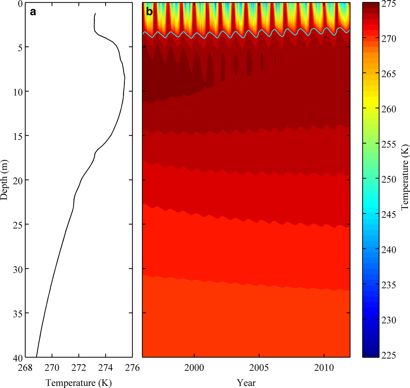
Fig. 6. (a) A typical water temperature profile from WLB (data obtained on 21 November 2011). (b) Modeled evolution of water temperature profile between 1996 and 2012.
For Lake Fryxell, the model was forced with meteorological data from the Lake Fryxell basin (Fig. 1). However, Lake Fryxell ice morphology (and the ice thickness) is significantly different than that of WLB and parameters related to optical properties of the ice required adjustment. As such, κ and χ were parameterized (increased) during the simulation. Albedo data for Lake Fryxell are not available and values used for WLB simulations were incorporated. Predicted ice thicknesses for Lake Fryxell show a good measured vs. modeled correlation of r = 0.90 (p < 0.001) and RMSE of 0.21 m (Fig. 7).
Fig. 7. Predicted ice thickness changes for Lake Fryxell (solid curve) and averaged measured ice thickness (circles) from 1996 to 2012. Numerous ice thickness measurements were obtained during the same day, showing large variability. Days with multiple ice thickness measurements were averaged. Error bars are shown as standard deviation. The curve that does not show seasonal cycle represents a spline fit to measured data, excluding late season 2008 measurements.
6. MODEL SENSITIVITY
The model sensitivity was tested by increasing/decreasing variables input by 10% of their nominal value, one at a time. The only exception is air temperature for which instead, the sensitivity was tested by an increase/decrease of 1°K. A simple modified sensitivity index (Si) was adapted from Hoffmann and Gardner (Reference Hoffmann and Gardner1983):
 $$Si = \left \vert {1 - \left( {\displaystyle{{D_{min}} \over {D_{max}}}} \right)} \right \vert $$
where D min is model output (ice thickness) when a variable was decreased, and D max is the model output when a variable was increased. Sensitivity index values range from 0 to 1, where 1 represents high sensitivity to a change in a parameter; values <0.01 indicate no sensitivity (Hoffmann and Gardner, Reference Hoffmann and Gardner1983). Each test was run over a 16 a period or until the ice cover melted, whichever came first. The sensitivity test was performed on shortwave radiation (Q s ), air temperature (T a ), bulk transfer coefficients (C E and C H ), albedo (α), extinction coefficient (κ) and a parameter responsible for partitioning shortwave radiation at the surface of the ice (χ). Sensitivity indices (Si) for each parameter are summarized in Table 1, from highest to lowest, and selected parameters are briefly discussed below.
Table 1. Sensitivity index (Si) results for parameters used in the model
Values <0.01 represent no sensitivity to the changes, whereas Si of 1 indicates large sensitivity to changes. χ is wavelength depended absorption of shortwave radiation at the surface of the ice, α is albedo, Q s is shortwave radiation, T a is air temperature, C E is bulk transfer coefficient used in latent heat equation, C H is bulk transfer coefficient used in the sensible heat equation, κ is extinction coefficient.
Shortwave radiation is the largest contributor of the energy at the very surface of the ice. As such, the output of the model is highly sensitive to parameters controlling shortwave radiation, including absorption (χ) and reflectance (α) (Table 1). For example, an increase of χ or α decreases solar radiation that penetrates an ice cover, decreasing the overall energy of the system that otherwise would be available for ice melt. This suggests the model is highly sensitive to parameters controlling surface optical properties of the ice. Q s and T a have an inverse effect on the ice cover thickness. An increase of Q s and T a significantly contributes to the surface ice temperature, as well as penetrating solar radiation, both of which will enhance melt.
The model is relatively insensitive to changes in bulk transfer coefficients (C E and C H , respectively). Changes in C E create small variations in the model's output (yet preserving the long-term trends), whereas changes in C H make virtually no difference to the output (Table 1). Similar sensitivity results were found by Vincent and others (Reference Vincent, Mueller and Vincent2008). The sensitivity test validates our original assumption of constant bulk transfer coefficients, reducing the computational complexity of the model.
Lake ice thickness is controlled by the surface energy balance and is presumed to reflect climatic changes (Wharton and others, Reference Wharton1992; Reid and Crout, Reference Reid and Crout2008). Taylor Valley experienced a general cooling trend between 1986 and 1999 (0.7 °C (10 a)−1), associated with increasing lake ice thickness (0.11 m a−1) and increasing shortwave radiation (8.1 W m−2 (10 a)−1), based on meteorological data from the Lake Hoare basin (Doran and others, Reference Doran2002b). Since early- to mid-2000, the increasing ice-thickness trends reversed: WLB ice thickness started to decrease in 2002 (Fig. 4) whereas the ice thickness of Lake Fryxell started to decline in 2006 (Fig. 7). The most notable change in the Taylor Valley climate during this time period was an exceptionally warm summer season during 2001/02 when maximum air temperature was >9°C (Barrett and others, Reference Barrett2008; Doran and others, Reference Doran2008).
The influence of seasonal temperature extremes on the long-term ice thickness trends is explored below. A sensitivity experiment was designed where the exceptionally warm season meteorological data of 2001/02 were substituted with meteorological data from an unusually cold season from the year prior (for WLB). The simulation results show no changes in the ice thickness trend (r = 0.98, p < 0.001). Conversely, the unusually cold season meteorological data, from a previous year, were randomly forced in the model during the ice thickness decline to test whether it would influence the long-term ice thickness trends. No changes in the trends were detected following this forcing, indicating that the long-term ice thickness trends in Taylor Valley lakes are not particularly responsive to discrete warming/cooling events. Rather, water column heat flux plays a major role in regulating ice thickness of the study lakes.
7. DISCUSSION
Predictions of long-term ice thickness trends of stratified perennially ice-covered lakes must consider the unique temperature profile of the water column of a lake as an additional heat source. In Antarctica's perennially ice-covered lakes, heat accumulates in the water column due to the continuous influx of solar radiation during austral summers (Shirtcliffe and Benseman, Reference Shirtcliffe and Benseman1964; Chinn, Reference Chinn, Green and Friedmann1993). The deep water temperature maximum associated with higher salt content takes decades to develop (Vincent and others, Reference Vincent, Mueller and Vincent2008).
Thermal structures of water columns can influence long-term ice thickness trends and preclude a response of the ice thickness to climatic changes. The water column temperature in Taylor Valley lakes is controlled by penetrating solar radiation (Shirtcliffe and Benseman, Reference Shirtcliffe and Benseman1964; Spigel and Priscu, Reference Spigel, Priscu and Priscu1998; Vincent and others, Reference Vincent, Mueller and Vincent2008). Penetrating solar radiation decays with depth in the ice and the water column based on the extinction coefficients. As a result, shallow water receives more energy than deep water and it will be more responsive to seasonal variations of penetrating solar radiation. Additionally, shallow water temperature is influenced by the contribution of sensible heat flux from the seasonal stream input, which enhances ice thinning. However, this is not included in the model. The energy stored at depth (long-term storage) will affect shallow water temperature, to a certain extent, by the upward heat conduction due to the thermal gradient. As a conceptual example, for a deep lake with a temperature maximum at some depth, during a climate cooling trend (assuming constant shortwave radiation), shallow waters will cool, increasing ice growth rates. Yet, shallow water will cool at rates slower than that of the air due to an influx of heat from the deep lake heat storage. The incoming heat from beneath will hinder shallow water cooling and slow ice thickness growth (e.g. Fig. 8). Conversely, for shallow lakes that do not have a deep temperature maximum, this process will be less pronounced and the shallow water temperature will more closely reflect climate cooling (Fig. 9). The situation would reverse during climate warming; the ice thickness of deep lakes with a well-developed temperature maximum would respond to surface air warming quicker due to the additional heat flux from beneath. For example, the ice thickness of WLB responded earlier to the increase of surface air temperature (Figs 4, 8) between 2000 and 2012 in comparison with ice thickness of Lake Fryxell (Figs 7, 9). This suggests that lakes with deep temperature maxima can reduce the response of ice thickness to climatic changes.
Fig. 8. Modeled temperature of the shallow water (bold solid curve), beneath the ice (4 m depth), over time at WLB and modeled ice thickness change over time (dashed curve). Shallow water temperature and ice thickness changes are inversely proportional.
Fig. 9. Modeled temperature of the shallow water (bold solid curve), beneath the ice (6 m depth), over time at Lake Fryxell and modeled ice thickness change over time (dashed curve). Shallow water temperature and ice thickness changes are inversely proportional.
The modeled water temperature profile of WLB shows three distinct trends: a continuous increase of deep water temperature over time, a continuous decrease of temperature maximum at ~9 m depth (Fig. 6), and a shallow water temperature (immediately beneath the ice) that varies inversely with the ice thickness (r = −0.85, p < 0.001) (Fig. 8). Annually measured temperature profiles of WLB show similar trends (unpublished data (John Priscu)). The only exception in measured data is an increase of temperature maximum after 2009, which is not captured by the model. The cooling of shallow water is associated with an ice thickness increase from 1996 to the end of 2001 (Fig. 8). Conversely, the warming of shallow water is associated with an ice thickness decrease after 2001 (Fig. 8). A similar trend of inversely proportional ice thickness and shallow water temperature is observed at Lake Fryxell; however, a clear temporal change in ice thickness and water temperature occurred in 2005 (Fig. 9). The difference in response time of the ice thickness in these two lakes can be attributed to the different thermal structures of the water columns near the ice/water interface, which is influenced by the deep thermal heat storage.
The observed long-term ice thickness trends in both lakes are a result, first and foremost, of the thermal structure of the water column and surface energy balance. The infrequent seasonal temperature increases do not influence long-term ice thickness trends because a secondary process (heat flux from the water column) that is driven on much longer timescales, influences the long-term trends of ice thickness. The alteration of the ice thickness trend occurs at a threshold dictated by heat fluxes at the ice surface and shallow water temperature, which is influenced by the thermal structure of the water column. Shallow water temperature is controlled by the penetrating shortwave radiation and the heat flux from deep waters. As a result, lake ice thickness will respond to climate forcings on different timescales depending on the thermal structure of the lake in question. We suggest that shallow perennially ice-covered lakes, such as Lake Fryxell, are a better proxy for climate change, owing to the fact that the ice thickness response to long-term climate forcing is not affected by the deep thermal water maximum.
8. CONCLUSIONS
A thermodynamic model parameterized for ice cover of WLB was developed. The model is driven by surface radiative heat fluxes and heat fluxes from the underlying water column, coupled with two 1-D heat equations. The water temperature profile is calculated in order to properly constrain heat fluxes at the ice/water boundary. Despite the simplistic nature of the model (it does not account for physics associated with isothermal ice, advection of the water column or sensible heat associated with stream inflow), the model successfully calculates long-term ice thickness changes as well as the temperature profile of the ice and the water column in two stratified lakes. Predicted ice thickness changes are in good agreement with trends observed in measured ice thickness data.
Perennially ice-covered lakes with a deep-water temperature maximum will impede the response of ice thickness growth to surface air cooling. The impact of surface air cooling is hindered by the heat flux from the water column. Conversely, during surface air warming, the water temperature maximum facilitates ice decay, due to an additional heat flux from below. Ice thickness of shallow lakes (<20 m), on the other hand, will more accurately respond to climatic changes because of diminished effect of the water column temperature on the ice thickness. Hence, ice covers can be used as indicators of climate change; however, the ice thickness trends should be interpreted with caution due to the influence of thermal stratification of the water column.
ACKNOWLEDGEMENTS
This research was supported by the Office of Polar Programs (grants 9810219, 0096250, 0832755, 1041742 and 1115245). Logistical support was provided by the US Antarctic Program through funding from NSF. We thank the Long Term Ecological Research project personnel for collecting the ice thickness measurements throughout the duration of this project and Douglas MacAyeal for insightful conversations on the topic.
APPENDIX


 Open access