1 Introduction
Turbulence is a process whereby energy injected into a system (via some mechanism usually associated with the system being out of equilibrium) is transferred nonlinearly – and therefore leading to chaotic and multiscale states – from the scale(s) at which it is injected to much smaller scales at which it is thermalised through microphysical dissipation channels available in the system. The system is forced to seek ways of transferring energy across a range of scales because the injection and dissipation physics are usually unrelated to each other and operate at disparate scales. It is the bridging of the gap between these scales that brings about turbulent cascades, broad-range power-law spectra and so on. In fluid systems, however varied and multiphysics they are, most turbulence theories are basically extensions and generalisations of the ideas of Richardson (Reference Richardson1922) and Kolmogorov (Reference Kolmogorov1941b ) of a local-in-scale cascade maintaining a constant flux of energy away from the injection and towards the dissipation scales (e.g. Zakharov, L’vov & Falkovich Reference Zakharov, L’vov and Falkovich1992; Davidson Reference Davidson2013). This type of thinking has been tremendously successful in making sense of experimental and numerical evidence in both fluids and plasmas.
In plasmas, however, a straightforward application of such ‘fluid’ thinking to any physical regime that is not collisionally dominated skirts over the obvious complication that the kinetic phase space includes the particle velocities as well as their positions, and the (free) energy is generally free to travel across this entire 6-D space. Its ability – and propensity – to do so is, in fact, manifest in what is probably the most important phenomenon that makes plasmas conceptually different from fluids – the Landau (Reference Landau1946) damping of electromagnetic perturbations in a collisionless plasma. Viewed in energy terms, it involves the transfer of free energy from electromagnetic perturbations into perturbations of the particle distribution function, which develops ever finer structure in velocity space (‘phase mixing’) until this transfer (which looks like damping if one only tracks the electromagnetic fields) is made irreversible by coarse graining of the velocity-space structure. The physical agent of this coarse graining is collisions, even if they would appear to be infinitesimally small. Mathematically, the Landau (Reference Landau1936) collision operator is a diffusion operator in velocity space and so even small collision frequencies are enough to thermalise any amount of energy, provided sufficiently large velocity-space gradients develop.
In a linear plasma system, Landau damping, or, more generally, phase mixing, is the only available thermalisation route. It provides an adequate mechanism to process any injected free energy at any fixed wavenumber (since the process is linear, energy will stay in the wavenumber into which it is injected; there is no coupling), leading to a finite effective damping rate and filling up the phase space with free energy. If one uses a Hermite decomposition to quantify ‘scales’ in velocity space, one finds that, in a steady-state system continuously pumped via low Hermite moments and dissipating free energy via high ones, the free energy will accumulate in phase space to a level that diverges if the collisionality is taken to zero; the collisional heating rate in this limit is finite and equal to the phase-mixing rate (Kanekar et al. Reference Kanekar, Schekochihin, Dorland and Loureiro2015). How does this mechanism coexist and compete with the refinement of spatial scales caused by coupling between scales – an inevitable consequence of nonlinearity?
In this paper, we address this question using a simple archetypal example of plasma turbulence–electrostatic turbulence in a drift-kinetic plasma. We will describe this example in § 2, along with all the relevant preliminaries: the concept of free energy, the Hermite decomposition, and the existing Kolmogorov-style ‘fluid’ turbulence theory for this problem (Barnes, Parra & Schekochihin Reference Barnes, Parra and Schekochihin2011). In § 3, we will introduce the phase-space formalism that explicitly separates the phase-mixing and the ‘anti-phase-mixing’ perturbations (the latter activated by the plasma echo effect), both of which turn out to be inevitable in a nonlinear system, and provides a useful starting point for a substantive theoretical treatment of phase-space turbulence. In § 4, a phenomenological scaling theory of this turbulence will be proposed. While we will describe in detail how free energy and its fluxes are distributed in the inertial range – leading to some interesting and testable scalings – the main conclusion will be that phase mixing is quite heavily suppressed in a turbulent system. Section 5 is devoted to summarising this and other findings and to discussing their implications, as well as future directions of research. A reader only interested in a digest can skip directly to this section.
2 Preliminaries
This section contains a rather extended tutorial on a number of topics constituting elementary but necessary background to what will follow. Readers who are sufficiently steeped in these matters can skim through this section and then dedicate themselves more seriously to §§ 3 and 4 (where references to relevant parts of § 2 will be supplied).
2.1 Prototypical kinetic problem
We consider a plasma near Maxwellian equilibrium, in which case the distribution function for particles of species $s$
can be expressed as
$s$
can be expressed as
 $$\begin{eqnarray}\displaystyle f_{s}=F_{Ms}+{\it\delta}f_{s}, & & \displaystyle\end{eqnarray}$$
where $F_{Ms}$
is a Maxwellian distribution and
$F_{Ms}$
is a Maxwellian distribution and ${\it\delta}f_{s}$
a small perturbation.
${\it\delta}f_{s}$
a small perturbation.
We assume this plasma to be in a uniform strong magnetic field $\boldsymbol{B}=B\hat{\boldsymbol{z}}$
(
$\boldsymbol{B}=B\hat{\boldsymbol{z}}$
( $\hat{\boldsymbol{z}}$
is the unit vector in the direction of this field, designated the
$\hat{\boldsymbol{z}}$
is the unit vector in the direction of this field, designated the $z$
axis). We consider low-frequency perturbations, which will be highly anisotropic with respect to the field:
$z$
axis). We consider low-frequency perturbations, which will be highly anisotropic with respect to the field:
 $$\begin{eqnarray}\displaystyle {\it\omega}\ll {\it\Omega}_{s},\quad k_{\Vert }\ll k_{\bot }, & & \displaystyle\end{eqnarray}$$
where ${\it\Omega}_{s}$
is the Larmor frequency.
${\it\Omega}_{s}$
is the Larmor frequency.
We assume these perturbations to be electrostatic, viz.,
 $$\begin{eqnarray}\displaystyle {\it\delta}\boldsymbol{E}=-\boldsymbol{{\rm\nabla}}{\it\phi},\quad {\it\delta}\boldsymbol{B}=0, & & \displaystyle\end{eqnarray}$$
where ${\it\phi}$
is the scalar potential. We use Gaussian electromagnetic units.
${\it\phi}$
is the scalar potential. We use Gaussian electromagnetic units.
We consider only long wavelengths,
 $$\begin{eqnarray}\displaystyle k_{\bot }{\it\rho}_{s}\ll 1, & & \displaystyle\end{eqnarray}$$
where ${\it\rho}_{s}$
is the Larmor radius.
${\it\rho}_{s}$
is the Larmor radius.
Finally, we assume a Boltzmann electron response (which arises via expansion of the electron drift-kinetic equation in the electron-to-ion mass ratio):Footnote 1
 $$\begin{eqnarray}\displaystyle \frac{e{\it\phi}}{T_{e}}=\frac{{\it\delta}n_{e}}{n_{e}}=\frac{{\it\delta}n_{i}}{n_{i}}=\frac{1}{n_{i}}\int \text{d}^{3}v{\it\delta}f_{i}, & & \displaystyle\end{eqnarray}$$
where $e$
is the electron charge,
$e$
is the electron charge, $T_{s}$
and
$T_{s}$
and $n_{s}$
are the equilibrium temperatures and number densities, respectively, and
$n_{s}$
are the equilibrium temperatures and number densities, respectively, and ${\it\delta}n_{s}$
are density perturbations (
${\it\delta}n_{s}$
are density perturbations ( $s=e$
for electrons,
$s=e$
for electrons, $s=i$
for ions). The second equality in (2.5) is a consequence of plasma quasineutrality. It is useful to denote
$s=i$
for ions). The second equality in (2.5) is a consequence of plasma quasineutrality. It is useful to denote
 $$\begin{eqnarray}\displaystyle {\it\varphi}=\frac{Ze{\it\phi}}{T_{i}}, & & \displaystyle\end{eqnarray}$$
where $Z$
is the ratio of the ion to electron charge.
$Z$
is the ratio of the ion to electron charge.
Under these assumptions, we may integrate out the dependence of the ion distribution function on perpendicular velocities, so we introduce
 $$\begin{eqnarray}\displaystyle g(t,\boldsymbol{r},v_{\Vert })=\frac{1}{n_{i}}\int \text{d}^{2}\boldsymbol{v}_{\bot }{\it\delta}f_{i}, & & \displaystyle\end{eqnarray}$$
and write the drift-kinetic equation for $g$
in a 4-D phase space:
$g$
in a 4-D phase space:
 $$\begin{eqnarray}\displaystyle & \displaystyle \frac{\partial g}{\partial t}+v_{\Vert }\boldsymbol{{\rm\nabla}}_{\Vert }(g+{\it\varphi}F_{M})+\boldsymbol{u}_{\bot }\boldsymbol{\cdot }\boldsymbol{{\rm\nabla}}_{\bot }g=C[g]+{\it\chi}, & \displaystyle\end{eqnarray}$$
 $$\begin{eqnarray}\displaystyle & \displaystyle {\it\varphi}={\it\alpha}\int \text{d}v_{\Vert }g,\quad {\it\alpha}=\frac{ZT_{e}}{T_{i}}, & \displaystyle\end{eqnarray}$$ $F_{M}$
is a 1-D Maxwellian with thermal speed
$F_{M}$
is a 1-D Maxwellian with thermal speed $v_{th}$
,
$v_{th}$
,  $$\begin{eqnarray}\displaystyle F_{M}=\frac{1}{\sqrt{{\rm\pi}}}\text{e}^{-v_{\Vert }^{2}/v_{th}^{2}},\quad v_{th}=\sqrt{\frac{2T_{i}}{m_{i}}}, & & \displaystyle\end{eqnarray}$$ $\boldsymbol{u}_{\bot }$
is the
$\boldsymbol{u}_{\bot }$
is the $\boldsymbol{E}\times \boldsymbol{B}$
drift velocity,
$\boldsymbol{E}\times \boldsymbol{B}$
drift velocity,
 $$\begin{eqnarray}\displaystyle \boldsymbol{u}_{\bot }=c\frac{{\it\delta}\boldsymbol{E}\times \boldsymbol{B}}{B^{2}}=\frac{{\it\rho}_{i}v_{th}}{2}\hat{\boldsymbol{z}}\times \boldsymbol{{\rm\nabla}}_{\bot }{\it\varphi}, & & \displaystyle\end{eqnarray}$$ $C[g]$
is the collision operator and
$C[g]$
is the collision operator and ${\it\chi}$
a source term – both of which need a little further discussion, which we will provide in § 2.1.2.
${\it\chi}$
a source term – both of which need a little further discussion, which we will provide in § 2.1.2.
Note that while we will be referring to ‘slab’ ion-temperature-gradient (ITG) turbulence (e.g. Cowley, Kulsrud & Sudan Reference Cowley, Kulsrud and Sudan1991; Ottaviani et al. Reference Ottaviani, Beer, Cowley, Horton and Krommes1997; Horton Reference Horton1999) as the main physical instantiation that we have in mind of the kinetic problem described above, there will be nothing in our theory that would make it inapplicable to the (inertial range of) electron-temperature-gradient (ETG) turbulence (Dorland et al. Reference Dorland, Jenko, Kotschenreuther and Rogers2000; Jenko et al. Reference Jenko, Dorland, Kotschenreuther and Rogers2000), or indeed to a generic case of electrostatic drift-kinetic turbulence with energy injection at long wavelengths.
2.1.1 A nuance: Boltzmann closure and zonal flows
In this context, we must come clean on an important detail. The Boltzmann closure (2.5) for the electron density is, in fact, only valid for perturbations with $k_{\Vert }\neq 0$
because it relies on electrons streaming quickly along the magnetic field lines to short out the parallel electric field. In tokamak plasmas, where magnetic shear imposes a link between
$k_{\Vert }\neq 0$
because it relies on electrons streaming quickly along the magnetic field lines to short out the parallel electric field. In tokamak plasmas, where magnetic shear imposes a link between $k_{\Vert }$
and
$k_{\Vert }$
and $k_{y}$
, the Boltzmann closure is normally amended (Dorland & Hammett Reference Dorland and Hammett1993; Hammett et al.
Reference Hammett, Beer, Dorland, Cowley and Smith1993) to remove from the electron density the response associated with perturbations that have
$k_{y}$
, the Boltzmann closure is normally amended (Dorland & Hammett Reference Dorland and Hammett1993; Hammett et al.
Reference Hammett, Beer, Dorland, Cowley and Smith1993) to remove from the electron density the response associated with perturbations that have $k_{y}=k_{\Vert }=0$
(the ‘zonal flows’), namely,
$k_{y}=k_{\Vert }=0$
(the ‘zonal flows’), namely,
 $$\begin{eqnarray}\displaystyle \frac{{\it\delta}n_{e}}{n_{e}}=\frac{e({\it\phi}-\overline{{\it\phi}})}{T_{e}}, & & \displaystyle\end{eqnarray}$$
where $\overline{{\it\phi}}$
is the flux-surface average, which in our context is an average over
$\overline{{\it\phi}}$
is the flux-surface average, which in our context is an average over $y$
and
$y$
and $z$
(formally, one obtains this by first deriving the density response in a toroidal, magnetically sheared system, as is done, e.g. in § J.2 of Abel & Cowley (Reference Abel and Cowley2013), then taking the magnetic shear and curvature to be small and passing to the slab limit).
$z$
(formally, one obtains this by first deriving the density response in a toroidal, magnetically sheared system, as is done, e.g. in § J.2 of Abel & Cowley (Reference Abel and Cowley2013), then taking the magnetic shear and curvature to be small and passing to the slab limit).
This implies that, in order to find the $(y,z)$
-averaged (zonal) part of
$(y,z)$
-averaged (zonal) part of ${\it\varphi}$
from the ion distribution function, at least the lowest-order finite-Larmor-radius correction has to be kept (physically representing the polarisation drift; see Krommes (Reference Krommes1993, Reference Krommes2010)), leading to
${\it\varphi}$
from the ion distribution function, at least the lowest-order finite-Larmor-radius correction has to be kept (physically representing the polarisation drift; see Krommes (Reference Krommes1993, Reference Krommes2010)), leading to ${\it\alpha}$
in (2.9) for the zonal part of
${\it\alpha}$
in (2.9) for the zonal part of ${\it\varphi}$
having to be replaced with
${\it\varphi}$
having to be replaced with ${\it\alpha}=2/k_{x}^{2}{\it\rho}_{i}^{2}$
, or
${\it\alpha}=2/k_{x}^{2}{\it\rho}_{i}^{2}$
, or
 $$\begin{eqnarray}\displaystyle -\frac{1}{2}\,{\it\rho}_{i}^{2}\partial _{x}^{2}\overline{{\it\varphi}}=\int \text{d}v_{\Vert }\overline{g}. & & \displaystyle\end{eqnarray}$$
In ITG turbulence far from marginal stability, these changes affect important quantitative details of the interaction between zonal flows and drift waves at the outer scale (Rogers, Dorland & Kotschenreuther (Reference Rogers, Dorland and Kotschenreuther2000); see also discussion around (2.43)), but do not matter for the inertial-range physics that we will focus on in this paper.
A reader who is unconvinced may observe that (2.9) can be used without these modifications if, instead of considering ITG turbulence, we consider ETG turbulence (Dorland et al. Reference Dorland, Jenko, Kotschenreuther and Rogers2000; Jenko et al. Reference Jenko, Dorland, Kotschenreuther and Rogers2000). In this case, it is the ions that have a Boltzmann response (due to their large Larmor orbits, over which the density response from electron-scale fluctuations averages out),
 $$\begin{eqnarray}\displaystyle \frac{{\it\delta}n_{i}}{n_{i}}=-\frac{Ze{\it\phi}}{T_{i}} & & \displaystyle\end{eqnarray}$$
(which is $={\it\delta}n_{e}/n_{e}$
by quasineutrality). The required modifications in (2.8) and (2.9) are
$={\it\delta}n_{e}/n_{e}$
by quasineutrality). The required modifications in (2.8) and (2.9) are
 $$\begin{eqnarray}\displaystyle {\it\varphi}\rightarrow \frac{e{\it\phi}}{T_{e}},\quad {\it\alpha}\rightarrow -\frac{T_{i}}{ZT_{e}},\quad {\it\rho}_{i}\rightarrow {\it\rho}_{e},\quad v_{th}\rightarrow v_{the}=\sqrt{\frac{2T_{e}}{m_{e}}}, & & \displaystyle\end{eqnarray}$$
and ${\it\varphi}F_{M}\rightarrow -{\it\varphi}F_{M}$
in (2.8). None of this affects anything essential in the upcoming theoretical developments.
${\it\varphi}F_{M}\rightarrow -{\it\varphi}F_{M}$
in (2.8). None of this affects anything essential in the upcoming theoretical developments.
2.1.2 Injection, phase mixing, advection and dissipation
The precise nature of the source term ${\it\chi}$
in (2.8) will not matter in our theory, as long as it does not contain any sharp dependence on
${\it\chi}$
in (2.8) will not matter in our theory, as long as it does not contain any sharp dependence on $v_{\Vert }$
(i.e. is confined to low velocity moments). A random forcing is often a convenient choice for analytical theory (e.g. Plunk Reference Plunk2013; Plunk & Parker Reference Plunk and Parker2014; Kanekar et al.
Reference Kanekar, Schekochihin, Dorland and Loureiro2015), but a more physical form in the context of electrostatic drift-kinetic turbulence in plasmas (e.g. Horton Reference Horton1999) arises from accounting for the presence of equilibrium density and temperature gradients, taken conventionally to be in the negative
$v_{\Vert }$
(i.e. is confined to low velocity moments). A random forcing is often a convenient choice for analytical theory (e.g. Plunk Reference Plunk2013; Plunk & Parker Reference Plunk and Parker2014; Kanekar et al.
Reference Kanekar, Schekochihin, Dorland and Loureiro2015), but a more physical form in the context of electrostatic drift-kinetic turbulence in plasmas (e.g. Horton Reference Horton1999) arises from accounting for the presence of equilibrium density and temperature gradients, taken conventionally to be in the negative $x$
direction:Footnote
2
$x$
direction:Footnote
2
 $$\begin{eqnarray}\displaystyle \begin{array}{@{}c@{}}\displaystyle {\it\chi}=-\frac{\boldsymbol{u}_{\bot }\boldsymbol{\cdot }\boldsymbol{{\rm\nabla}}(n_{i}F_{M})}{n_{i}}=-\frac{{\it\rho}_{i}v_{th}}{2}\frac{\partial {\it\varphi}}{\partial y}\left[\frac{1}{L_{n}}+\left(\frac{v_{\Vert }^{2}}{v_{th}^{2}}-\frac{1}{2}\right)\frac{1}{L_{T}}\right]F_{M},\\ \displaystyle \frac{1}{L_{n}}=-\frac{1}{n_{i}}\frac{\text{d}n_{i}}{\text{d}x},\quad \frac{1}{L_{T}}=-\frac{1}{T_{i}}\frac{\text{d}T_{i}}{\text{d}x}.\end{array} & & \displaystyle\end{eqnarray}$$
We shall see in § 2.3 that these terms render the system linearly unstable and thus extract energy from the equilibrium gradients and inject it into the perturbed distribution.
The resulting perturbations are subject to two influences, linear and nonlinear, encoded by the second ( $v_{\Vert }\boldsymbol{{\rm\nabla}}_{\Vert }g$
) and fourth (
$v_{\Vert }\boldsymbol{{\rm\nabla}}_{\Vert }g$
) and fourth ( $\boldsymbol{u}_{\bot }\boldsymbol{\cdot }\boldsymbol{{\rm\nabla}}_{\bot }g$
) terms on the left-hand side of (2.8), respectively. The nonlinear term represents advection of the distribution function by the mean perpendicular flow, itself determined by the former. This involves coupling between different wavenumbers and thus usually leads to spatial mixing (generation of small spatial scales) of the perturbed distribution. The linear term represents phase mixing – generation of small velocity-space scales in the perturbed distribution function. The simplest way to understand this is to notice that the homogeneous solution to the linear kinetic equation in Fourier space,
$\boldsymbol{u}_{\bot }\boldsymbol{\cdot }\boldsymbol{{\rm\nabla}}_{\bot }g$
) terms on the left-hand side of (2.8), respectively. The nonlinear term represents advection of the distribution function by the mean perpendicular flow, itself determined by the former. This involves coupling between different wavenumbers and thus usually leads to spatial mixing (generation of small spatial scales) of the perturbed distribution. The linear term represents phase mixing – generation of small velocity-space scales in the perturbed distribution function. The simplest way to understand this is to notice that the homogeneous solution to the linear kinetic equation in Fourier space, $\partial _{t}g+\text{i}v_{\Vert }k_{\Vert }g=\cdots \,,$
is
$\partial _{t}g+\text{i}v_{\Vert }k_{\Vert }g=\cdots \,,$
is $g\sim \text{e}^{-\text{i}v_{\Vert }k_{\Vert }t}$
and the velocity gradient of that grows secularly with time,
$g\sim \text{e}^{-\text{i}v_{\Vert }k_{\Vert }t}$
and the velocity gradient of that grows secularly with time, $\partial _{v_{\Vert }}g=-\text{i}k_{\Vert }tg$
.
$\partial _{v_{\Vert }}g=-\text{i}k_{\Vert }tg$
.
As fine structure in phase space is generated, there must be a means for removing it. This is why, even for a ‘collisionless’ (meaning in fact weakly collisional) plasma, the collision operator $C[g]$
must be included in (2.8). We hasten to acknowledge that, in pretending that the collision operator operates purely on
$C[g]$
must be included in (2.8). We hasten to acknowledge that, in pretending that the collision operator operates purely on $g$
, we are ignoring that the
$g$
, we are ignoring that the $\boldsymbol{v}_{\bot }$
dependence cannot in fact be integrated out of it: collisions will strive to isotropise the distribution and so the collision operator must necessarily couple
$\boldsymbol{v}_{\bot }$
dependence cannot in fact be integrated out of it: collisions will strive to isotropise the distribution and so the collision operator must necessarily couple $\boldsymbol{v}_{\bot }$
and
$\boldsymbol{v}_{\bot }$
and $v_{\Vert }$
. However, non-rigorously, when the collision frequency is small,
$v_{\Vert }$
. However, non-rigorously, when the collision frequency is small,
 $$\begin{eqnarray}\displaystyle {\it\nu}\ll {\it\omega},k_{\Vert }v_{th},k_{\bot }u_{\bot }, & & \displaystyle\end{eqnarray}$$
the collision operator’s essential contribution will be simply to iron out fine structure in velocity space and, given an initial distribution and a source that are smooth in $\boldsymbol{v}$
, only fine structure in
$\boldsymbol{v}$
, only fine structure in $v_{\Vert }$
can arise. Thus, it should suffice to assume a simple model form for
$v_{\Vert }$
can arise. Thus, it should suffice to assume a simple model form for $C[g]$
: for example, the Lenard & Bernstein (Reference Lenard and Bernstein1958) operator,
$C[g]$
: for example, the Lenard & Bernstein (Reference Lenard and Bernstein1958) operator,
 $$\begin{eqnarray}\displaystyle C[g]={\it\nu}\frac{\partial }{\partial \hat{v}_{\Vert }}\left(\frac{1}{2}\frac{\partial }{\partial \hat{v}_{\Vert }}+\hat{v}_{\Vert }\right)g,\quad \hat{v}_{\Vert }=\frac{v_{\Vert }}{v_{th}}. & & \displaystyle\end{eqnarray}$$
The fact that this operator does not conserve momentum or energy, while easily repaired if one strives for quantitatively precise energetics (Kirkwood Reference Kirkwood1946), will not cause embarrassment as collisions will only matter for high velocity moments (because large gradients with respect to $v_{\Vert }$
are necessary to offset the smallness of
$v_{\Vert }$
are necessary to offset the smallness of ${\it\nu}$
). It is not hard to estimate the velocity-space scales at which collisions can become important: balancing
${\it\nu}$
). It is not hard to estimate the velocity-space scales at which collisions can become important: balancing $C[g]\sim {\it\omega}g$
, where
$C[g]\sim {\it\omega}g$
, where ${\it\omega}\sim k_{\Vert }v_{th}$
and/or
${\it\omega}\sim k_{\Vert }v_{th}$
and/or $k_{\bot }u_{\bot }$
is the typical frequency scale of the collisionless dynamics, we find that the requisite velocity scale is
$k_{\bot }u_{\bot }$
is the typical frequency scale of the collisionless dynamics, we find that the requisite velocity scale is
 $$\begin{eqnarray}\displaystyle \frac{{\it\delta}v_{\Vert }}{v_{th}}\sim \left(\frac{{\it\nu}}{{\it\omega}}\right)^{1/2}, & & \displaystyle\end{eqnarray}$$
so the structure gets ever finer as ${\it\nu}\rightarrow +0$
.
${\it\nu}\rightarrow +0$
.
Finally, we are going to assume implicitly that (2.8) contains some regularising term to ensure a cutoff in $k_{\bot }$
– a necessity because of the spatial mixing associated with the nonlinear advection. Physically, the advection term will drive the system out of the domain of validity of the drift-kinetic approximation, to
$k_{\bot }$
– a necessity because of the spatial mixing associated with the nonlinear advection. Physically, the advection term will drive the system out of the domain of validity of the drift-kinetic approximation, to $k_{\bot }{\it\rho}_{i}\sim 1$
and larger. The precise way in which the energy is thermalised at these Larmor and sub-Larmor scales is a rich and interesting topic in its own right, involving a kinetic cascade in a 5-D phase space (with nonlinear phase mixing in
$k_{\bot }{\it\rho}_{i}\sim 1$
and larger. The precise way in which the energy is thermalised at these Larmor and sub-Larmor scales is a rich and interesting topic in its own right, involving a kinetic cascade in a 5-D phase space (with nonlinear phase mixing in $v_{\bot }$
now also occurring) – but these matters are outside the scope of this treatment (see Schekochihin et al.
Reference Schekochihin, Cowley, Dorland, Hammett, Howes, Plunk, Quataert and Tatsuno2008, Reference Schekochihin, Cowley, Dorland, Hammett, Howes, Quataert and Tatsuno2009; Tatsuno et al.
Reference Tatsuno, Dorland, Schekochihin, Plunk, Barnes, Cowley and Howes2009; Plunk et al.
Reference Plunk, Cowley, Schekochihin and Tatsuno2010; Bañón Navarro et al.
Reference Bañón Navarro, Morel, Albrecht-Marc, Carati, Merz, Görler and Jenko2011b
).
$v_{\bot }$
now also occurring) – but these matters are outside the scope of this treatment (see Schekochihin et al.
Reference Schekochihin, Cowley, Dorland, Hammett, Howes, Plunk, Quataert and Tatsuno2008, Reference Schekochihin, Cowley, Dorland, Hammett, Howes, Quataert and Tatsuno2009; Tatsuno et al.
Reference Tatsuno, Dorland, Schekochihin, Plunk, Barnes, Cowley and Howes2009; Plunk et al.
Reference Plunk, Cowley, Schekochihin and Tatsuno2010; Bañón Navarro et al.
Reference Bañón Navarro, Morel, Albrecht-Marc, Carati, Merz, Görler and Jenko2011b
).
It is the competition between the two ways – linear phase mixing versus nonlinear advection – of generating small-scale structure in phase space thus enabling the energy injected by the source to be thermalised that will be the subject of this paper.
2.2 Free energy
We have referred to injection and thermalisation of energy many times now, and so defining precisely what we mean by ‘energy’ has become overdue.
Energy in ${\it\delta}f$
kinetics (i.e. in near-equilibrium kinetics) is the free energy associated with the perturbed distribution:Footnote
3
${\it\delta}f$
kinetics (i.e. in near-equilibrium kinetics) is the free energy associated with the perturbed distribution:Footnote
3
 $$\begin{eqnarray}\displaystyle {\mathcal{F}}=-\mathop{\sum }_{s}T_{s}{\it\delta}S_{s}=\mathop{\sum }_{s}T_{s}{\it\delta}\int \text{d}^{3}\boldsymbol{v}\langle f_{s}\ln f_{s}\rangle =\mathop{\sum }_{s}\int \text{d}^{3}\boldsymbol{v}\frac{T_{s}\langle {\it\delta}f_{s}^{2}\rangle }{2F_{Ms}}, & & \displaystyle\end{eqnarray}$$
where angle brackets denote spatial averaging and ${\it\delta}S_{s}$
is the mean additional (negative!) entropy associated with the perturbed distribution of species
${\it\delta}S_{s}$
is the mean additional (negative!) entropy associated with the perturbed distribution of species $s$
. The last expression in (2.20) was obtained by letting
$s$
. The last expression in (2.20) was obtained by letting $f_{s}=F_{Ms}+{\it\delta}f_{s}$
and expanding
$f_{s}=F_{Ms}+{\it\delta}f_{s}$
and expanding $\langle f_{s}\ln f_{s}\rangle$
to second order in
$\langle f_{s}\ln f_{s}\rangle$
to second order in ${\it\delta}f_{s}$
(see, e.g. Schekochihin et al.
Reference Schekochihin, Cowley, Dorland, Hammett, Howes, Plunk, Quataert and Tatsuno2008; note that
${\it\delta}f_{s}$
(see, e.g. Schekochihin et al.
Reference Schekochihin, Cowley, Dorland, Hammett, Howes, Plunk, Quataert and Tatsuno2008; note that $\langle {\it\delta}f_{s}\rangle =0$
because
$\langle {\it\delta}f_{s}\rangle =0$
because $\langle f_{s}\rangle =F_{Ms}$
by definition). It is now not hard to establish that
$\langle f_{s}\rangle =F_{Ms}$
by definition). It is now not hard to establish that ${\mathcal{F}}=n_{i}T_{i}W$
, where
${\mathcal{F}}=n_{i}T_{i}W$
, where
 $$\begin{eqnarray}\displaystyle W=\int \text{d}v_{\Vert }\frac{\langle g^{2}\rangle }{2F_{M}}+\frac{\langle {\it\varphi}^{2}\rangle }{2{\it\alpha}} & & \displaystyle\end{eqnarray}$$
is the quadratic quantity conserved by (2.8). This can be shown either by using the Boltzmann-electron closure in (2.20) (viz., ${\it\delta}f_{e}=(e{\it\phi}/T_{e})F_{Me}$
, so the
${\it\delta}f_{e}=(e{\it\phi}/T_{e})F_{Me}$
, so the $s=e$
term in
$s=e$
term in $\sum _{s}$
gives rise to the
$\sum _{s}$
gives rise to the $\langle {\it\varphi}^{2}\rangle$
term in
$\langle {\it\varphi}^{2}\rangle$
term in $W$
) or directly starting from (2.8), which gives us the following law of evolution of the free energy:
$W$
) or directly starting from (2.8), which gives us the following law of evolution of the free energy:
 $$\begin{eqnarray}\displaystyle \frac{\text{d}W}{\text{d}t}=\int \text{d}v_{\Vert }\left(\frac{\langle g{\it\chi}\rangle }{F_{M}}+\langle {\it\varphi}{\it\chi}\rangle \right)+\int \text{d}v_{\Vert }\frac{\langle gC[g]\rangle }{F_{M}}. & & \displaystyle\end{eqnarray}$$
The first term on the right-hand side is the energy-injection term, which turns into the usual flux term for ITG (or ETG) turbulence if we substitute ${\it\chi}$
from (2.16) (see (2.37)), and the second, negative definite, term is the collisional thermalisation of this energy flux.
${\it\chi}$
from (2.16) (see (2.37)), and the second, negative definite, term is the collisional thermalisation of this energy flux.
The Landau damping of the electrostatic perturbations is simply the transfer of free energy, via phase mixing, from the $\langle {\it\varphi}^{2}\rangle$
part of
$\langle {\it\varphi}^{2}\rangle$
part of $W$
to
$W$
to $\langle g^{2}\rangle$
Footnote
4
: since
$\langle g^{2}\rangle$
Footnote
4
: since ${\it\varphi}={\it\alpha}\int \text{d}v_{\Vert }g$
, small-scale velocity-space structure in
${\it\varphi}={\it\alpha}\int \text{d}v_{\Vert }g$
, small-scale velocity-space structure in $g$
is washed out in
$g$
is washed out in ${\it\varphi}$
but of course remains as free energy in
${\it\varphi}$
but of course remains as free energy in $\langle g^{2}\rangle$
(cf. Hammett & Perkins Reference Hammett and Perkins1990; Hammett, Dorland & Perkins Reference Hammett, Dorland and Perkins1992).
$\langle g^{2}\rangle$
(cf. Hammett & Perkins Reference Hammett and Perkins1990; Hammett, Dorland & Perkins Reference Hammett, Dorland and Perkins1992).
2.3 Hermite decomposition
A natural way to separate the ‘fluid’ part of the problem from the ‘kinetic’ part and represent phase mixing is to expand the perturbed distribution in Hermite polynomials:Footnote 5
 $$\begin{eqnarray}\displaystyle & \displaystyle g(v_{\Vert })=\mathop{\sum }_{m=0}^{\infty }\frac{H_{m}(\hat{v}_{\Vert })F_{M}(v_{\Vert })}{\sqrt{2^{m}m!}}g_{m}, & \displaystyle\end{eqnarray}$$
 $$\begin{eqnarray}\displaystyle & \displaystyle g_{m}=\int \text{d}v_{\Vert }\frac{H_{m}(\hat{v}_{\Vert })}{\sqrt{2^{m}m!}}g(v_{\Vert }), & \displaystyle\end{eqnarray}$$ $\hat{v}_{\Vert }=v_{\Vert }/v_{th}$
and the ‘physicist’s’ Hermite polynomials are
$\hat{v}_{\Vert }=v_{\Vert }/v_{th}$
and the ‘physicist’s’ Hermite polynomials are  $$\begin{eqnarray}\displaystyle H_{m}(\hat{v}_{\Vert })=(-1)^{m}\text{e}^{\hat{v}_{\Vert }^{2}}\frac{\text{d}^{m}}{\text{d}\hat{v}_{\Vert }^{m}}\text{e}^{-\hat{v}_{\Vert }^{2}},\quad \int \text{d}v_{\Vert }\frac{H_{m}(\hat{v}_{\Vert })H_{n}(\hat{v}_{\Vert })}{2^{m}m!}F_{M}(v_{\Vert })={\it\delta}_{mn}. & & \displaystyle\end{eqnarray}$$
The first three Hermite moments are the (ion) density ( ${\it\delta}n$
), mean-parallel-velocity (
${\it\delta}n$
), mean-parallel-velocity ( $u_{\Vert }$
) and parallel-temperature (
$u_{\Vert }$
) and parallel-temperature ( ${\it\delta}T_{\Vert }$
) perturbations:
${\it\delta}T_{\Vert }$
) perturbations:
 $$\begin{eqnarray}\displaystyle \displaystyle H_{0}(\hat{v}_{\Vert })=1 & \quad \Rightarrow \quad & \displaystyle \displaystyle g_{0}=\frac{{\it\delta}n}{n}=\frac{{\it\varphi}}{{\it\alpha}},\end{eqnarray}$$
 $$\begin{eqnarray}\displaystyle \displaystyle H_{1}(\hat{v}_{\Vert })=2\hat{v}_{\Vert } & \quad \Rightarrow \quad & \displaystyle \displaystyle g_{1}=\sqrt{2}\,\frac{u_{\Vert }}{v_{th}},\end{eqnarray}$$
 $$\begin{eqnarray}\displaystyle \displaystyle H_{2}(\hat{v}_{\Vert })=4\left(\hat{v}_{\Vert }^{2}-\frac{1}{2}\right) & \quad \Rightarrow \quad & \displaystyle \displaystyle g_{2}=\frac{1}{\sqrt{2}}\frac{{\it\delta}T_{\Vert }}{T}.\end{eqnarray}$$
 $$\begin{eqnarray}\displaystyle {\it\chi}=-\frac{{\it\rho}_{i}v_{th}}{2}\frac{\partial {\it\varphi}}{\partial y}\left[\frac{H_{0}(\hat{v}_{\Vert })}{L_{n}}+\frac{H_{2}(\hat{v}_{\Vert })}{4L_{T}}\right]F_{M}\equiv \left[{\it\chi}_{0}+\frac{H_{2}(\hat{v}_{\Vert })}{2\sqrt{2}}{\it\chi}_{2}\right]F_{M} & & \displaystyle\end{eqnarray}$$
and that the streaming term in (2.8), $v_{\Vert }\boldsymbol{{\rm\nabla}}_{\Vert }g$
, couples Hermite moments of adjacent orders via the formula
$v_{\Vert }\boldsymbol{{\rm\nabla}}_{\Vert }g$
, couples Hermite moments of adjacent orders via the formula
 $$\begin{eqnarray}\displaystyle \hat{v}_{\Vert }H_{m}(\hat{v}_{\Vert })={\textstyle \frac{1}{2}}H_{m+1}(\hat{v}_{\Vert })+mH_{m-1}(\hat{v}_{\Vert }), & & \displaystyle\end{eqnarray}$$
we arrive at the following Hermite representation of (2.8):
 $$\begin{eqnarray}\displaystyle & & \displaystyle \displaystyle \frac{\partial }{\partial t}\frac{{\it\varphi}}{{\it\alpha}}+v_{th}\boldsymbol{{\rm\nabla}}_{\Vert }\frac{u_{\Vert }}{v_{th}}={\it\chi}_{0}=-\frac{v_{th}}{2L_{n}}{\it\rho}_{i}\frac{\partial {\it\varphi}}{\partial y},\end{eqnarray}$$
 $$\begin{eqnarray}\displaystyle & & \displaystyle \displaystyle \left(\frac{\partial }{\partial t}+\boldsymbol{u}_{\bot }\boldsymbol{\cdot }\boldsymbol{{\rm\nabla}}_{\bot }\right)\frac{u_{\Vert }}{v_{th}}+v_{th}\boldsymbol{{\rm\nabla}}_{\Vert }\left(\frac{1}{2}\frac{{\it\delta}T_{\Vert }}{T}+\frac{1+{\it\alpha}}{{\it\alpha}}\,{\it\varphi}\right)=0,\end{eqnarray}$$
 $$\begin{eqnarray}\displaystyle & & \displaystyle \displaystyle \left(\frac{\partial }{\partial t}+\boldsymbol{u}_{\bot }\boldsymbol{\cdot }\boldsymbol{{\rm\nabla}}_{\bot }\right)\frac{{\it\delta}T_{\Vert }}{T}+v_{th}\boldsymbol{{\rm\nabla}}_{\Vert }\left(\sqrt{3}g_{3}+2\frac{u_{\Vert }}{v_{th}}\right)=\sqrt{2}{\it\chi}_{2}=-\frac{v_{th}}{2L_{T}}{\it\rho}_{i}\frac{\partial {\it\varphi}}{\partial y},\end{eqnarray}$$ $m\geqslant 3$
, a universal equation retaining no traces of the temperature-gradient drive or Boltzmann-electron physics:
$m\geqslant 3$
, a universal equation retaining no traces of the temperature-gradient drive or Boltzmann-electron physics:  $$\begin{eqnarray}\displaystyle \left(\frac{\partial }{\partial t}+\boldsymbol{u}_{\bot }\boldsymbol{\cdot }\boldsymbol{{\rm\nabla}}_{\bot }\right)g_{m}+v_{th}\boldsymbol{{\rm\nabla}}_{\Vert }\left(\sqrt{\frac{m+1}{2}}g_{m+1}+\sqrt{\frac{m}{2}}g_{m-1}\right)=-{\it\nu}mg_{m}. & & \displaystyle\end{eqnarray}$$
Note that we have taken advantage of the fact that Hermite polynomials are eigenfunctions of the Lenard–Bernstein operator (2.18), but ignored collisions in the $m=1$
and
$m=1$
and $m=2$
equations (this is allowed because we are assuming
$m=2$
equations (this is allowed because we are assuming ${\it\nu}\rightarrow +0$
and so collisions will only be important at
${\it\nu}\rightarrow +0$
and so collisions will only be important at $m\gg 1$
).
$m\gg 1$
).
2.3.1 Energy injection: slab ITG instability
The first three equations are the standard three-field fluid system that describes an ITG-unstable plasma at long wavelengths in an unsheared slab (Cowley et al. Reference Cowley, Kulsrud and Sudan1991). The quickest way to obtain the slab ITG instability (Rudakov & Sagdeev Reference Rudakov and Sagdeev1961; Coppi, Rosenbluth & Sagdeev Reference Coppi, Rosenbluth and Sagdeev1967; Cowley et al. Reference Cowley, Kulsrud and Sudan1991) is to balance the two terms on the left-hand side of (2.31), the first with the third term in (2.32) and the first term on the left-hand side with the temperature-gradient term on the right-hand side of (2.33). The resulting dispersion relation has three roots, of which one is unstable:
 $$\begin{eqnarray}\displaystyle {\it\omega}^{3}\approx \frac{{\it\alpha}}{2}(k_{\Vert }v_{th})^{2}{\it\omega}_{\ast T}\quad \Rightarrow \quad {\it\omega}\approx \left(-\frac{1}{2}+\text{i}\frac{\sqrt{3}}{2}\right)\left(\frac{{\it\alpha}}{2}\right)^{1/3}(k_{\Vert }v_{th})^{2/3}{\it\omega}_{\ast T}^{1/3}, & & \displaystyle\end{eqnarray}$$
where ${\it\omega}_{\ast T}=k_{y}{\it\rho}_{i}v_{th}/2L_{T}$
. This approximation is valid provided
${\it\omega}_{\ast T}=k_{y}{\it\rho}_{i}v_{th}/2L_{T}$
. This approximation is valid provided $L_{n}/L_{T}\gg 1$
and
$L_{n}/L_{T}\gg 1$
and ${\it\omega}_{\ast T}\gg k_{\Vert }v_{th}$
, although, as the growth rate grows with
${\it\omega}_{\ast T}\gg k_{\Vert }v_{th}$
, although, as the growth rate grows with $k_{\Vert }$
, the fastest growth is in fact achieved for
$k_{\Vert }$
, the fastest growth is in fact achieved for $k_{\Vert }v_{th}\sim {\it\omega}_{\ast T}$
, when the dispersion relation is a more complicated and somewhat unedifying equation. At
$k_{\Vert }v_{th}\sim {\it\omega}_{\ast T}$
, when the dispersion relation is a more complicated and somewhat unedifying equation. At $k_{\Vert }v_{th}\gg {\it\omega}_{\ast T}$
, the ITG mode is replaced by a sound wave, which, in a kinetic system, is heavily Landau damped.Footnote
6
$k_{\Vert }v_{th}\gg {\it\omega}_{\ast T}$
, the ITG mode is replaced by a sound wave, which, in a kinetic system, is heavily Landau damped.Footnote
6
2.3.2 Free-energy flows
The temperature-gradient instability injects energy into the ${\it\varphi}$
,
${\it\varphi}$
, $u_{\Vert }/v_{th}$
and
$u_{\Vert }/v_{th}$
and ${\it\delta}T_{\Vert }/T$
perturbations, all of which are comparable to each other in magnitude when
${\it\delta}T_{\Vert }/T$
perturbations, all of which are comparable to each other in magnitude when $k_{\Vert }v_{th}\sim {\it\omega}_{\ast T}$
. Because the three-field system is not closed,Footnote
7
there is a transfer of energy from
$k_{\Vert }v_{th}\sim {\it\omega}_{\ast T}$
. Because the three-field system is not closed,Footnote
7
there is a transfer of energy from ${\it\delta}T_{\Vert }/T$
to higher Hermite moments: the
${\it\delta}T_{\Vert }/T$
to higher Hermite moments: the $g_{3}$
term in (2.33) provides the energy sink from the unstable (‘forced’) moments and the
$g_{3}$
term in (2.33) provides the energy sink from the unstable (‘forced’) moments and the $g_{2}$
term in (2.34) at
$g_{2}$
term in (2.34) at $m=3$
is the source for the higher moments; the energy thus received by them is eventually thermalised via collisions.
$m=3$
is the source for the higher moments; the energy thus received by them is eventually thermalised via collisions.
To be more precise about these statements, let us rewrite the free energy (2.21) in terms of Hermite moments:
 $$\begin{eqnarray}\displaystyle W=\frac{1+{\it\alpha}}{2{\it\alpha}^{2}}\langle {\it\varphi}^{2}\rangle +\frac{\langle u_{\Vert }^{2}\rangle }{v_{th}^{2}}+\frac{1}{4}\frac{\langle {\it\delta}T_{\Vert }^{2}\rangle }{T^{2}}+\frac{1}{2}\mathop{\sum }_{m=3}^{\infty }\langle g_{m}^{2}\rangle . & & \displaystyle\end{eqnarray}$$
Its ‘fluid’ and ‘kinetic’ parts satisfy:Footnote 8
 $$\begin{eqnarray}\displaystyle & & \displaystyle \displaystyle \frac{\text{d}}{\text{d}t}\left(\frac{1+{\it\alpha}}{{\it\alpha}^{2}}\langle {\it\varphi}^{2}\rangle +\frac{\langle u_{\Vert }^{2}\rangle }{v_{th}^{2}}+\frac{1}{4}\frac{\langle {\it\delta}T_{\Vert }^{2}\rangle }{T^{2}}\right)=\frac{\langle {\it\delta}T_{\Vert }u_{x}\rangle }{2TL_{T}}-\frac{\sqrt{3}v_{th}}{2T}\langle {\it\delta}T_{\Vert }\boldsymbol{{\rm\nabla}}_{\Vert }g_{3}\rangle ,\end{eqnarray}$$
 $$\begin{eqnarray}\displaystyle & & \displaystyle \displaystyle \frac{\text{d}}{\text{d}t}\frac{1}{2}\mathop{\sum }_{m=3}^{\infty }\langle g_{m}^{2}\rangle =\frac{\sqrt{3}v_{th}}{2T}\langle {\it\delta}T_{\Vert }\boldsymbol{{\rm\nabla}}_{\Vert }g_{3}\rangle -{\it\nu}\mathop{\sum }_{m=3}^{\infty }m\langle g_{m}^{2}\rangle .\end{eqnarray}$$ $\text{d}\langle \cdots \!\rangle /\text{d}t=0$
, we must have
$\text{d}\langle \cdots \!\rangle /\text{d}t=0$
, we must have  $$\begin{eqnarray}\displaystyle \langle {\it\delta}T_{\Vert }\boldsymbol{{\rm\nabla}}_{\Vert }g_{3}\rangle \geqslant 0 & & \displaystyle\end{eqnarray}$$
because the collision term is negative definite in (2.38), and, therefore,
 $$\begin{eqnarray}\displaystyle \langle {\it\delta}T_{\Vert }u_{x}\rangle \geqslant 0 & & \displaystyle\end{eqnarray}$$
to achieve balance in (2.37). The inequality (2.39) implies a non-negative mean energy flux to higher Hermite moments (cf. Krommes & Hu Reference Krommes and Hu1994; Nakata, Watanabe & Sugama Reference Nakata, Watanabe and Sugama2012).
How that flux is processed from being injected at $m=3$
to being dissipated at
$m=3$
to being dissipated at $m\gg 1$
(assuming
$m\gg 1$
(assuming ${\it\nu}\rightarrow +0$
) is handled by (2.34). This equation contains in a beautifully explicit form the two effects to which this paper is devoted: the phase mixing is manifest in that
${\it\nu}\rightarrow +0$
) is handled by (2.34). This equation contains in a beautifully explicit form the two effects to which this paper is devoted: the phase mixing is manifest in that $g_{m}$
is coupled to
$g_{m}$
is coupled to $g_{m+1}$
and
$g_{m+1}$
and $g_{m-1}$
, providing a mechanism for pushing energy to higher
$g_{m-1}$
, providing a mechanism for pushing energy to higher $m$
’s; simultaneously, all Hermite moments
$m$
’s; simultaneously, all Hermite moments $g_{m}$
are advected (spatially mixed towards smaller scales) by the same fluctuating velocity
$g_{m}$
are advected (spatially mixed towards smaller scales) by the same fluctuating velocity $\boldsymbol{u}_{\bot }$
, determined, via (2.11), by the zeroth Hermite moment,
$\boldsymbol{u}_{\bot }$
, determined, via (2.11), by the zeroth Hermite moment, ${\it\varphi}={\it\alpha}g_{0}$
.
${\it\varphi}={\it\alpha}g_{0}$
.
2.4 ‘Fluid’ turbulence theory
Barnes et al. (Reference Barnes, Parra and Schekochihin2011) proposed a Kolmogorov-style theory of ITG turbulence, essentially ignoring the possibility of a leakage of free energy from the low Hermite moments to the high. While their theory is by no means uncontroversial or the only offering on the market (e.g. Gürcan et al. Reference Gürcan, Garbet, Hennequin, Diamond, Casati and Falchetto2009; Plunk, Bañón Navarro & Jenko Reference Plunk, Bañón Navarro and Jenko2015), it does appear to match the results of numerical experiments (in the strongly unstable regime) and so it is worth both reviewing how it is constructed and examining to what extent it contradicts the statement made in the previous subsection that free energy must leak to higher Hermite moments.
The scaling argument of Barnes et al. (Reference Barnes, Parra and Schekochihin2011) addresses two main questions (as would any such argument aspiring to be a complete theory):
-
(i) what is the effective outer (energy-containing) scale of the turbulence and the fluctuation level at that scale;
-
(ii) what is the spatial structure of the turbulence in the ‘inertial range’ between that outer scale and the small-scale cutoff?
2.4.1 Outer scale
The first question would be trivial for turbulence forced externally at some fixed scale, but for temperature-gradient-driven turbulence, relying on a linear instability, the system must decide where to have its energy-containing scale. This is not simply the peak scale of the growth rate because at long wavelengths the growth rate will generally grow with wavenumber less quickly than will the nonlinear cascade rate (as we shall see in § 2.4.2) and so in fact it is the largest scale at which there is an instability that will end up being the energy-containing scale.
Barnes et al. (Reference Barnes, Parra and Schekochihin2011) conjectured that this infrared cutoff will be set by the largest parallel scale available to fluctuations:
 $$\begin{eqnarray}\displaystyle k_{\Vert 0}\sim \frac{1}{L_{\Vert }}, & & \displaystyle\end{eqnarray}$$
where $L_{\Vert }$
in our idealised homogeneous system is simply the parallel extent of the ‘box’ – in a tokamak, it would be the magnetic connection length between unstable and stable parts of the plasma (
$L_{\Vert }$
in our idealised homogeneous system is simply the parallel extent of the ‘box’ – in a tokamak, it would be the magnetic connection length between unstable and stable parts of the plasma ( $L_{\Vert }\sim qR$
, where
$L_{\Vert }\sim qR$
, where $q$
is safety factor and
$q$
is safety factor and $R$
the major radius). The perpendicular energy-containing scale is then given by
$R$
the major radius). The perpendicular energy-containing scale is then given by
 $$\begin{eqnarray}\displaystyle {\it\omega}_{\ast T}=k_{y0}{\it\rho}_{i}\frac{v_{th}}{L_{T}}\sim k_{\Vert 0}v_{th}\quad \Rightarrow \quad k_{y0}{\it\rho}_{i}\sim \frac{L_{T}}{L_{\Vert }} & & \displaystyle\end{eqnarray}$$
because the instability would be supplanted by stable (in fact, Landau damped) sound waves at smaller $k_{y}$
. Note that we require
$k_{y}$
. Note that we require $L_{T}/L_{\Vert }\ll 1$
for the turbulence to occur in a scale range consistent with the drift-kinetic approximation
$L_{T}/L_{\Vert }\ll 1$
for the turbulence to occur in a scale range consistent with the drift-kinetic approximation $k_{\bot }{\it\rho}_{i}\ll 1$
. Finally, it is further conjectured that the zonal flows generated by the turbulence will have a typical shearing rate
$k_{\bot }{\it\rho}_{i}\ll 1$
. Finally, it is further conjectured that the zonal flows generated by the turbulence will have a typical shearing rate $S_{ZF}$
comparable to the nonlinear decorrelation rate
$S_{ZF}$
comparable to the nonlinear decorrelation rate ${\it\tau}_{nl0}^{-1}$
at the outer scale (cf. Rogers et al.
Reference Rogers, Dorland and Kotschenreuther2000) and, therefore, will isotropise the turbulence:Footnote
9
${\it\tau}_{nl0}^{-1}$
at the outer scale (cf. Rogers et al.
Reference Rogers, Dorland and Kotschenreuther2000) and, therefore, will isotropise the turbulence:Footnote
9
 $$\begin{eqnarray}\displaystyle k_{x0}\sim S_{ZF}k_{y0}{\it\tau}_{nl0}\sim k_{y0}\sim k_{\bot 0}. & & \displaystyle\end{eqnarray}$$
This is the only place in the theory where the zonal flows make an appearance as it is assumed that they do not completely dominate the nonlinear dynamics, in contrast to their alleged behaviour in the near-threshold regime (e.g. Dimits et al. Reference Dimits, Bateman, Beer, Cohen, Dorland, Hammett, Kim, Kinsey, Kotschenreuther and Kritz2000; Diamond et al. Reference Diamond, Itoh, Itoh and Hahm2005; Diamond, Hasegawa & Mima Reference Diamond, Hasegawa and Mima2011; Gürcan et al. Reference Gürcan, Garbet, Hennequin, Diamond, Casati and Falchetto2009; Nakata et al. Reference Nakata, Watanabe and Sugama2012; Ghim et al. Reference Ghim, Schekochihin, Field, Abel, Barnes, Colyer, Cowley, Parra, Dunai and Zoletnik2013; Connaughton, Nazarenko & Quinn Reference Connaughton, Nazarenko and Quinn2014; Makwana et al. Reference Makwana, Terry, Pueschel and Hatch2014).
The energy-containing scale given by (2.42), the amount of energy it contains is estimated by balancing the rate of injection by instability, ${\it\omega}_{\ast T}$
, against the rate
${\it\omega}_{\ast T}$
, against the rate ${\it\tau}_{nl0}^{-1}$
of nonlinear removal of this energy to smaller scales via advection by the turbulent flow:
${\it\tau}_{nl0}^{-1}$
of nonlinear removal of this energy to smaller scales via advection by the turbulent flow:
 $$\begin{eqnarray}\displaystyle {\it\omega}_{\ast T}\sim k_{\bot 0}{\it\rho}_{i}\frac{v_{th}}{L_{T}}\sim {\it\tau}_{nl0}^{-1}\sim k_{\bot 0}u_{\bot 0}\sim {\it\rho}_{i}v_{th}k_{\bot 0}^{2}{\it\varphi}_{0}\quad \Rightarrow \quad {\it\varphi}_{0}\sim \frac{1}{k_{\bot 0}L_{T}}\sim \frac{{\it\rho}_{i}L_{\Vert }}{L_{T}^{2}}. & & \displaystyle\end{eqnarray}$$
Finally, if one’s overriding practical concern is the calculation of the effective heat transport caused by the turbulence, one concludes from the above that the turbulent thermal diffusivity and the heat flux are
 $$\begin{eqnarray}\displaystyle D_{turb}\sim u_{\bot 0}^{2}{\it\tau}_{nl0}\sim \frac{u_{\bot 0}}{k_{\bot 0}}\sim {\it\rho}_{i}v_{th}{\it\varphi}_{0},\quad \Rightarrow \quad Q\sim \frac{nD_{turb}T}{L_{T}}\sim n{\it\rho}_{i}^{2}v_{th}\,\frac{L_{\Vert }}{L_{T}^{3}}. & & \displaystyle\end{eqnarray}$$
All of this is not particularly sensitive to the fact that, in making the argument that led to (2.44), we completely ignored the possibility (in fact, the inevitability) that some of the energy injected at the outer scale might be removed not by the nonlinear advection, as if the system were purely fluid, but also by the phase mixing towards high $m$
’s. The presence of such a transfer (of which there is, in fact, numerical evidence; see, e.g. Watanabe & Sugama Reference Watanabe and Sugama2006, Hatch et al.
Reference Hatch, Terry, Jenko, Merz and Nevins2011a
,Reference Hatch, Terry, Jenko, Merz, Pueschel, Nevins and Wang
b
, Nakata et al.
Reference Nakata, Watanabe and Sugama2012) would only break our argument if the rate
$m$
’s. The presence of such a transfer (of which there is, in fact, numerical evidence; see, e.g. Watanabe & Sugama Reference Watanabe and Sugama2006, Hatch et al.
Reference Hatch, Terry, Jenko, Merz and Nevins2011a
,Reference Hatch, Terry, Jenko, Merz, Pueschel, Nevins and Wang
b
, Nakata et al.
Reference Nakata, Watanabe and Sugama2012) would only break our argument if the rate ${\sim}k_{\Vert 0}v_{th}$
of this transfer were substantially larger than the nonlinear-advection rate and so if the dominant balance were
${\sim}k_{\Vert 0}v_{th}$
of this transfer were substantially larger than the nonlinear-advection rate and so if the dominant balance were ${\it\omega}_{\ast T}\sim k_{\Vert 0}v_{th}\gg k_{\bot 0}u_{\bot 0}$
. But this is obviously impossible as one cannot saturate a linear instability by a linear mechanism: there would not be anything in the theory to determine the saturated amplitude.Footnote
10
In view of (2.42), the phase mixing rate is, in fact, of the same order as both
${\it\omega}_{\ast T}\sim k_{\Vert 0}v_{th}\gg k_{\bot 0}u_{\bot 0}$
. But this is obviously impossible as one cannot saturate a linear instability by a linear mechanism: there would not be anything in the theory to determine the saturated amplitude.Footnote
10
In view of (2.42), the phase mixing rate is, in fact, of the same order as both ${\it\omega}_{\ast T}$
and
${\it\omega}_{\ast T}$
and $k_{\bot 0}u_{\bot 0}$
. Therefore, it cannot affect the basic scalings – although for the purposes of quantitative transport modelling, it is quite crucial to know by what fraction of order unity it might cut the nonlinear mixing rate, a key preoccupation in the development of ‘Landau-fluid’ closures for plasma turbulence in fusion contexts (Hammett et al.
Reference Hammett, Dorland and Perkins1992, Reference Hammett, Beer, Dorland, Cowley and Smith1993; Dorland & Hammett Reference Dorland and Hammett1993; Beer & Hammett Reference Beer and Hammett1996; Snyder & Hammett Reference Snyder and Hammett2001b
).
$k_{\bot 0}u_{\bot 0}$
. Therefore, it cannot affect the basic scalings – although for the purposes of quantitative transport modelling, it is quite crucial to know by what fraction of order unity it might cut the nonlinear mixing rate, a key preoccupation in the development of ‘Landau-fluid’ closures for plasma turbulence in fusion contexts (Hammett et al.
Reference Hammett, Dorland and Perkins1992, Reference Hammett, Beer, Dorland, Cowley and Smith1993; Dorland & Hammett Reference Dorland and Hammett1993; Beer & Hammett Reference Beer and Hammett1996; Snyder & Hammett Reference Snyder and Hammett2001b
).
A question that is much more sensitive to whether phase mixing is non-negligible is the structure of the inertial range.
2.4.2 Inertial range: perpendicular spectrum
How is the energy injected at $(k_{\bot 0},k_{\Vert 0})$
cascaded to smaller scales? Ignoring phase mixing, Barnes et al. (Reference Barnes, Parra and Schekochihin2011) proposed to calculate the dependence of the turbulent amplitudes on scale via the Kolmogorov assumption of constant energy flux: at each scale
$(k_{\bot 0},k_{\Vert 0})$
cascaded to smaller scales? Ignoring phase mixing, Barnes et al. (Reference Barnes, Parra and Schekochihin2011) proposed to calculate the dependence of the turbulent amplitudes on scale via the Kolmogorov assumption of constant energy flux: at each scale $k_{\bot }^{-1}$
, energy
$k_{\bot }^{-1}$
, energy ${\it\varphi}^{2}$
is transferred (locally) to the next smaller scale over the cascade time
${\it\varphi}^{2}$
is transferred (locally) to the next smaller scale over the cascade time ${\it\tau}_{nl}$
:
${\it\tau}_{nl}$
:
 $$\begin{eqnarray}\displaystyle \frac{{\it\varphi}^{2}}{{\it\tau}_{nl}}\sim k_{\bot }u_{\bot }{\it\varphi}^{2}\propto k_{\bot }^{2}{\it\varphi}^{3}=\text{const}\quad \Rightarrow \quad {\it\varphi}\propto k_{\bot }^{-2/3}, & & \displaystyle\end{eqnarray}$$
where we used $u_{\bot }\propto k_{\bot }{\it\varphi}$
(see (2.11)). Note that, both here and in similar arguments that will follow, we do not make a distinction between the energy content of low-
$u_{\bot }\propto k_{\bot }{\it\varphi}$
(see (2.11)). Note that, both here and in similar arguments that will follow, we do not make a distinction between the energy content of low- $m$
moments, assumingFootnote
11
$m$
moments, assumingFootnote
11
 $$\begin{eqnarray}\displaystyle {\it\varphi}\sim \frac{u_{\Vert }}{v_{th}}\sim \frac{{\it\delta}T_{\Vert }}{T} & & \displaystyle\end{eqnarray}$$
and possibly also ${\sim}$
a few more low-
${\sim}$
a few more low- $m$
moments of
$m$
moments of $g$
, although we do assume that there is not a substantial energy leakage to asymptotically large
$g$
, although we do assume that there is not a substantial energy leakage to asymptotically large $m$
’s. The 1-D (perpendicular) spectrum is then
$m$
’s. The 1-D (perpendicular) spectrum is then
 $$\begin{eqnarray}\displaystyle E_{{\it\varphi}}^{\bot }(k_{\bot })=2{\rm\pi}k_{\bot }\int \text{d}k_{\Vert }\langle |{\it\varphi}_{\boldsymbol{k}}|^{2}\rangle \sim \frac{{\it\varphi}^{2}}{k_{\bot }}\propto k_{\bot }^{-7/3}, & & \displaystyle\end{eqnarray}$$
where $\langle \cdots \rangle$
now denotes a time or ensemble average. This scaling is supported both by numerical simulations of Barnes et al. (Reference Barnes, Parra and Schekochihin2011) and, apparently, by those done by other groups (Hatch et al. (Reference Hatch, Jenko, Bañón Navarro and Bratanov2013, Reference Hatch, Jenko, Bratanov and Bañón Navarro2014), Plunk et al. (Reference Plunk, Bañón Navarro and Jenko2015) who confirm finding the same scaling, without, however, providing plots).
$\langle \cdots \rangle$
now denotes a time or ensemble average. This scaling is supported both by numerical simulations of Barnes et al. (Reference Barnes, Parra and Schekochihin2011) and, apparently, by those done by other groups (Hatch et al. (Reference Hatch, Jenko, Bañón Navarro and Bratanov2013, Reference Hatch, Jenko, Bratanov and Bañón Navarro2014), Plunk et al. (Reference Plunk, Bañón Navarro and Jenko2015) who confirm finding the same scaling, without, however, providing plots).
2.4.3 Critical balance
The structure of the turbulence in the parallel direction can now be inferred via a causality argument known in the astrophysical MHD literature as ‘critical balance’ (Goldreich & Sridhar Reference Goldreich and Sridhar1995, Reference Goldreich and Sridhar1997; Boldyrev Reference Boldyrev2005) and emerging as a universal scaling principle for strong turbulence in wave-supporting systems (Cho & Lazarian Reference Cho and Lazarian2004; Schekochihin et al. Reference Schekochihin, Cowley, Dorland, Hammett, Howes, Quataert and Tatsuno2009; Nazarenko & Schekochihin Reference Nazarenko and Schekochihin2011): fluctuations cannot stay correlated at parallel distances longer than those over which linear communication happens at the same rate as the nonlinear decorrelation: thus, fluctuations are uncorrelated for
 $$\begin{eqnarray}\displaystyle k_{\Vert }v_{th}\lesssim k_{\bot }u_{\bot }\propto k_{\bot }^{4/3}\quad \Rightarrow \quad k_{\Vert }L_{\Vert }\lesssim \left(\frac{k_{\bot }}{k_{\bot 0}}\right)^{4/3}. & & \displaystyle\end{eqnarray}$$
Here, and in what follows, we shall adopt a non-dimensionalisation $L_{\Vert }=1$
and
$L_{\Vert }=1$
and $k_{\bot 0}=1$
, so the above condition will henceforth be written
$k_{\bot 0}=1$
, so the above condition will henceforth be written $k_{\Vert }\lesssim k_{\bot }^{4/3}$
.
$k_{\Vert }\lesssim k_{\bot }^{4/3}$
.
This argument implies that, at any given $k_{\bot }$
, the ‘energy-containing’ parallel scale will be given by the ‘critical-balance’ wavenumber:
$k_{\bot }$
, the ‘energy-containing’ parallel scale will be given by the ‘critical-balance’ wavenumber:
 $$\begin{eqnarray}\displaystyle k_{\Vert c}v_{th}\sim k_{\bot }u_{\bot }\quad \Rightarrow \quad k_{\Vert c}\sim k_{\bot }^{4/3}, & & \displaystyle\end{eqnarray}$$
another scaling that was confirmed numerically by Barnes et al. (Reference Barnes, Parra and Schekochihin2011). The consequent scaling of the 1-D parallel spectrum is (using (2.50) in (2.46))Footnote 12
 $$\begin{eqnarray}\displaystyle {\it\varphi}\propto k_{\Vert }^{-1/2}\quad \Rightarrow \quad E_{{\it\varphi}}^{\Vert }(k_{\Vert })=2{\rm\pi}\int \text{d}k_{\bot }k_{\bot }\langle |{\it\varphi}_{\boldsymbol{k}}|^{2}\rangle \sim \frac{{\it\varphi}^{2}}{k_{\Vert }}\propto k_{\Vert }^{-2}. & & \displaystyle\end{eqnarray}$$
Note that, under this scheme, the drift waves are slow in the inertial range because ${\it\omega}_{\ast T}\propto k_{y}$
whereas
${\it\omega}_{\ast T}\propto k_{y}$
whereas $k_{\bot }u_{\bot }\propto k_{\bot }^{4/3}$
, so the relevant frequency in (2.49) is indeed
$k_{\bot }u_{\bot }\propto k_{\bot }^{4/3}$
, so the relevant frequency in (2.49) is indeed ${\sim}k_{\Vert }v_{th}$
, not
${\sim}k_{\Vert }v_{th}$
, not ${\it\omega}_{\ast T}$
. By the same token, energy injection by the temperature-gradient instability is slow compared to the nonlinear cascade rate, so, effectively, the instability only operates at the outer scale, while the fluctuations that carry the injected energy through the inertial range are more akin to ion sound waves than to drift waves.Footnote
13
${\it\omega}_{\ast T}$
. By the same token, energy injection by the temperature-gradient instability is slow compared to the nonlinear cascade rate, so, effectively, the instability only operates at the outer scale, while the fluctuations that carry the injected energy through the inertial range are more akin to ion sound waves than to drift waves.Footnote
13
2.4.4 Constant flux is inconsistent with robust phase mixing
In § 4.2, we will explain how to derive from these arguments the scaling of the 2-D spectra for any $k_{\bot }$
and
$k_{\bot }$
and $k_{\Vert }$
. However, we must first discuss the key point that the constant-flux assumption (2.46) cannot be consistent with both the idea that the energy resides along the ‘critical-balance curve’ (2.50) and with phase mixing taking energy out to large
$k_{\Vert }$
. However, we must first discuss the key point that the constant-flux assumption (2.46) cannot be consistent with both the idea that the energy resides along the ‘critical-balance curve’ (2.50) and with phase mixing taking energy out to large $m$
’s at the rate
$m$
’s at the rate ${\sim}k_{\Vert }v_{th}$
– simply because the latter would mean that the energy in the low-
${\sim}k_{\Vert }v_{th}$
– simply because the latter would mean that the energy in the low- $m$
moments is not conserved and so need not be fully transferred nonlinearly to smaller scales.
$m$
moments is not conserved and so need not be fully transferred nonlinearly to smaller scales.
The simplest way to explain the implications of this for the spectra is to replace (2.46) by a simple mock-up of an evolution equation for $E_{{\it\varphi}}^{\bot }(k_{\bot })$
(cf. Batchelor Reference Batchelor1953; Howes et al.
Reference Howes, Cowley, Dorland, Hammett, Quataert and Schekochihin2008):
$E_{{\it\varphi}}^{\bot }(k_{\bot })$
(cf. Batchelor Reference Batchelor1953; Howes et al.
Reference Howes, Cowley, Dorland, Hammett, Quataert and Schekochihin2008):
 $$\begin{eqnarray}\displaystyle \frac{\partial E_{{\it\varphi}}^{\bot }}{\partial t}=-\frac{\partial {\it\varepsilon}}{\partial k_{\bot }}-{\it\gamma}E_{{\it\varphi}}^{\bot },\quad {\it\varepsilon}\sim \frac{k_{\bot }E_{{\it\varphi}}^{\bot }}{{\it\tau}_{nl}},\quad {\it\gamma}\sim k_{\Vert }v_{th}\sim {\it\tau}_{nl}^{-1}\sim k_{\bot }^{2}\sqrt{k_{\bot }E_{{\it\varphi}}^{\bot }},\quad & & \displaystyle\end{eqnarray}$$
where ${\it\varepsilon}$
is the energy flux and
${\it\varepsilon}$
is the energy flux and ${\it\gamma}$
is the effective rate of phase mixing (Landau damping), which, by the critical-balance conjecture (2.50), is of the same order as the cascade rate
${\it\gamma}$
is the effective rate of phase mixing (Landau damping), which, by the critical-balance conjecture (2.50), is of the same order as the cascade rate ${\it\tau}_{nl}^{-1}$
. Assuming steady state in (2.52) and letting
${\it\tau}_{nl}^{-1}$
. Assuming steady state in (2.52) and letting ${\it\gamma}{\it\tau}_{nl}={\it\xi}=\text{const}\sim 1$
(independent of
${\it\gamma}{\it\tau}_{nl}={\it\xi}=\text{const}\sim 1$
(independent of $k_{\bot }$
, as per critical balance), we find
$k_{\bot }$
, as per critical balance), we find
 $$\begin{eqnarray}\displaystyle \frac{\partial {\it\varepsilon}}{\partial k_{\bot }}=-\frac{{\it\xi}}{k_{\bot }}\,{\it\varepsilon}\quad \Rightarrow \quad {\it\varepsilon}\propto k_{\bot }^{-{\it\xi}}\quad \Rightarrow \quad E_{{\it\varphi}}^{\bot }(k_{\bot })\propto k_{\bot }^{-(7+2{\it\xi})/3}. & & \displaystyle\end{eqnarray}$$
Thus, the flux decreases with increasing wavenumber and so the spectrum is steeper than the constant-flux solution (2.48). The power laws that emerge in such dissipative systems are generally hard to predict and probably non-universal (cf. Bratanov et al.
Reference Bratanov, Jenko, Hatch and Wilczek2013; Passot & Sulem Reference Passot and Sulem2015) – in our case, because they depend on an order-unity prefactor ( ${\it\xi}$
) in the critical-balance relation (2.50), rather than on some dimensionally and physically inevitable scaling.Footnote
14
However, numerical – or, indeed, experimental – evidence does not appear to support spectra that are significantly steeper than
${\it\xi}$
) in the critical-balance relation (2.50), rather than on some dimensionally and physically inevitable scaling.Footnote
14
However, numerical – or, indeed, experimental – evidence does not appear to support spectra that are significantly steeper than $k_{\bot }^{-2}$
at long (above the Larmor scale) wavelengths (e.g. Hennequin et al.
Reference Hennequin, Sabot, Honoré, Hoang, Garbet, Truc, Fenzi and Quéméneur2004; Görler & Jenko Reference Görler and Jenko2008; Casati et al.
Reference Casati, Gerbaud, Hennequin, Bourdelle, Candy, Clairet, Garbet, Grandgirard, Gürcan and Heuraux2009; Barnes et al.
Reference Barnes, Parra and Schekochihin2011; Vermare et al.
Reference Vermare, Hennequin, Gürcan, Bourdelle, Clairet, Garbet and Sabot2011; Kobayashi & Gürcan Reference Kobayashi and Gürcan2015). Furthermore, numerical investigations by Teaca et al. (Reference Teaca, Navarro, Jenko, Brunner and Villard2012), Teaca, Navarro & Jenko (Reference Teaca, Navarro and Jenko2014) and Bañón Navarro et al. (Reference Bañón Navarro, Teaca, Jenko, Hammett and Happel2014) confirm local nonlinear energy transfer and possibly even constant fluxes, albeit with a number of caveats regarding non-asymptoticity of the simulations, consequent possible non-universality of their results, as well as distinctly measurable, if not dominant, amounts of dissipation (meaning, in their context, phase mixing) everywhere.
$k_{\bot }^{-2}$
at long (above the Larmor scale) wavelengths (e.g. Hennequin et al.
Reference Hennequin, Sabot, Honoré, Hoang, Garbet, Truc, Fenzi and Quéméneur2004; Görler & Jenko Reference Görler and Jenko2008; Casati et al.
Reference Casati, Gerbaud, Hennequin, Bourdelle, Candy, Clairet, Garbet, Grandgirard, Gürcan and Heuraux2009; Barnes et al.
Reference Barnes, Parra and Schekochihin2011; Vermare et al.
Reference Vermare, Hennequin, Gürcan, Bourdelle, Clairet, Garbet and Sabot2011; Kobayashi & Gürcan Reference Kobayashi and Gürcan2015). Furthermore, numerical investigations by Teaca et al. (Reference Teaca, Navarro, Jenko, Brunner and Villard2012), Teaca, Navarro & Jenko (Reference Teaca, Navarro and Jenko2014) and Bañón Navarro et al. (Reference Bañón Navarro, Teaca, Jenko, Hammett and Happel2014) confirm local nonlinear energy transfer and possibly even constant fluxes, albeit with a number of caveats regarding non-asymptoticity of the simulations, consequent possible non-universality of their results, as well as distinctly measurable, if not dominant, amounts of dissipation (meaning, in their context, phase mixing) everywhere.
In what follows, we shall see that, in a sufficiently collisionless plasma, the constant-flux assumption is safer than it might appear.
2.5 Hermite ‘cascade’
As the final piece of essential background, let us consider what happens with free energy in phase space if we treat phase mixing as the dominant process and ignore nonlinearity – the opposite extreme to that pursued in § 2.4.
Returning to (2.34) and dropping the advection term $\boldsymbol{u}_{\bot }\boldsymbol{\cdot }\boldsymbol{{\rm\nabla}}_{\bot }$
for the time being, we perform a Fourier transform in the parallel direction and introduce the following very useful functions (Zocco & Schekochihin Reference Zocco and Schekochihin2011):
$\boldsymbol{u}_{\bot }\boldsymbol{\cdot }\boldsymbol{{\rm\nabla}}_{\bot }$
for the time being, we perform a Fourier transform in the parallel direction and introduce the following very useful functions (Zocco & Schekochihin Reference Zocco and Schekochihin2011):
 $$\begin{eqnarray}\displaystyle \tilde{g}_{m}(k_{\Vert })=(\text{i}\,\text{sgn}k_{\Vert })^{m}g_{m}(k_{\Vert }), & & \displaystyle\end{eqnarray}$$
where $g_{m}(k_{\Vert })$
are the Fourier–Hermite harmonics. The (linearised) equation (2.34) then becomes
$g_{m}(k_{\Vert })$
are the Fourier–Hermite harmonics. The (linearised) equation (2.34) then becomes
 $$\begin{eqnarray}\displaystyle \frac{\partial \tilde{g}_{m}}{\partial t}+\frac{|k_{\Vert }|v_{th}}{\sqrt{2}}(\sqrt{m+1}\tilde{g}_{m+1}-\sqrt{m}\tilde{g}_{m-1})=-{\it\nu}m\tilde{g}_{m}. & & \displaystyle\end{eqnarray}$$
The point of these manipulations is that they have made the phase-mixing term on the left-hand side of (2.55) look like a derivative with respect to $m$
. Indeed, assuming, in the limit of
$m$
. Indeed, assuming, in the limit of $m\gg 1$
, that we can treat
$m\gg 1$
, that we can treat $\tilde{g}_{m}$
as though it were continuous and differentiable in
$\tilde{g}_{m}$
as though it were continuous and differentiable in $m$
(an assumption that will come under close scrutiny in § 3.1), i.e.
$m$
(an assumption that will come under close scrutiny in § 3.1), i.e. $\tilde{g}_{m\pm 1}\approx \tilde{g}_{m}\pm \partial _{m}\tilde{g}_{m}$
, we have
$\tilde{g}_{m\pm 1}\approx \tilde{g}_{m}\pm \partial _{m}\tilde{g}_{m}$
, we have
 $$\begin{eqnarray}\displaystyle \sqrt{m+1}\tilde{g}_{m+1}-\sqrt{m}\tilde{g}_{m-1} & = & \displaystyle \sqrt{m}\left(\sqrt{1+\frac{1}{m}}\tilde{g}_{m+1}-\tilde{g}_{m-1}\right)\nonumber\\ \displaystyle & {\approx} & \displaystyle \sqrt{m}\left(\frac{\tilde{g}_{m}}{2m}+2\frac{\partial \tilde{g}_{m}}{\partial m}\right)=2m^{1/4}\frac{\partial }{\partial m}m^{1/4}\tilde{g}_{m}.\end{eqnarray}$$
Thus, (2.55) becomes
 $$\begin{eqnarray}\displaystyle \frac{\partial \tilde{g}_{m}}{\partial t}+\sqrt{2}|k_{\Vert }|v_{th}m^{1/4}\frac{\partial }{\partial m}m^{1/4}\tilde{g}_{m}=-{\it\nu}m\tilde{g}_{m}. & & \displaystyle\end{eqnarray}$$
Introducing the Fourier–Hermite free-energy spectrum $C_{m}(k_{\Vert })=\langle |\tilde{g}_{m}(k_{\Vert })|^{2}\rangle =\langle |g_{m}(k_{\Vert })|^{2}\rangle$
, we find
$C_{m}(k_{\Vert })=\langle |\tilde{g}_{m}(k_{\Vert })|^{2}\rangle =\langle |g_{m}(k_{\Vert })|^{2}\rangle$
, we find
 $$\begin{eqnarray}\displaystyle \frac{\partial C_{m}}{\partial t}+\frac{\partial }{\partial m}|k_{\Vert }|v_{th}\sqrt{2m}C_{m}=-2{\it\nu}mC_{m}. & & \displaystyle\end{eqnarray}$$
In steady state, the solution is (Zocco & Schekochihin Reference Zocco and Schekochihin2011; cf. Watanabe & Sugama Reference Watanabe and Sugama2004)
 $$\begin{eqnarray}\displaystyle C_{m}=\frac{A(k_{\Vert })}{\sqrt{m}}\text{e}^{-(m/m_{c})^{3/2}},\quad m_{c}=\left(\frac{3|k_{\Vert }|v_{th}}{2\sqrt{2}{\it\nu}}\right)^{2/3}, & & \displaystyle\end{eqnarray}$$
where $A(k_{\Vert })$
is the constant of integration. Below the collisional cutoff,
$A(k_{\Vert })$
is the constant of integration. Below the collisional cutoff, $m\ll m_{c}$
, the power-law scaling
$m\ll m_{c}$
, the power-law scaling $C_{m}\propto m^{-1/2}$
is the solution corresponding to constant free-energy flux in Hermite space (the Hermite flux is the expression under
$C_{m}\propto m^{-1/2}$
is the solution corresponding to constant free-energy flux in Hermite space (the Hermite flux is the expression under $\partial _{m}$
in (2.58)). It is possible to show quite rigorously (by direct Hermite transformation of the Landau response function) that this is indeed the Hermite-space solution that arises in a linear system with external forcing at low
$\partial _{m}$
in (2.58)). It is possible to show quite rigorously (by direct Hermite transformation of the Landau response function) that this is indeed the Hermite-space solution that arises in a linear system with external forcing at low $m$
and Landau damping (Kanekar et al.
Reference Kanekar, Schekochihin, Dorland and Loureiro2015).
$m$
and Landau damping (Kanekar et al.
Reference Kanekar, Schekochihin, Dorland and Loureiro2015).
The solution (2.59) has two important properties. Firstly, the free-energy dissipation associated with it (the last term in (2.38)) is dominated by Hermite moments with $m\sim m_{c}$
and does not explicitly depend on the collision frequency (assuming
$m\sim m_{c}$
and does not explicitly depend on the collision frequency (assuming $A(k_{\Vert })$
does not),
$A(k_{\Vert })$
does not),
 $$\begin{eqnarray}\displaystyle D={\it\nu}\mathop{\sum }_{m}m\langle g_{m}^{2}\rangle ={\it\nu}\mathop{\sum }_{k_{\Vert }}\mathop{\sum }_{m}mC_{m}(k_{\Vert })\approx {\it\nu}\mathop{\sum }_{k_{\Vert }}\int _{{\sim}1}^{\infty }\text{d}m\,mC_{m}(k_{\Vert })=\mathop{\sum }_{k_{\Vert }}\frac{|k_{\Vert }|v_{th}A(k_{\Vert })}{\sqrt{2}}. & & \displaystyle \nonumber\\ \displaystyle & & \displaystyle\end{eqnarray}$$
Secondly, the total amount of free energy stored in the phase space in order to achieve this finite dissipation (corresponding to finite amount of injected power) diverges as ${\it\nu}\rightarrow 0$
:
${\it\nu}\rightarrow 0$
:
 $$\begin{eqnarray}\displaystyle W\approx \frac{1}{2}\mathop{\sum }_{k_{\Vert }}\int _{{\sim}1}^{\infty }\text{d}m\,C_{m}(k_{\Vert })=\mathop{\sum }_{k_{\Vert }}\frac{{\it\Gamma}(1/3)}{3^{2/3}\sqrt{2}}\frac{A(k_{\Vert })}{(|k_{\Vert }|v_{th})^{2/3}{\it\nu}^{1/3}} & & \displaystyle\end{eqnarray}$$
(Kanekar et al. Reference Kanekar, Schekochihin, Dorland and Loureiro2015).
Thus, if we thought that Landau damping in a turbulent system works in the same way as it does in a linear one, we might have to conclude that, rather than staying in low $m$
’s and being nonlinearly cascaded to small spatial scales, as in a fluid problem, the free energy fills up phase space and dissipates in collisions. A dedicated study of the Hermite spectra of slab ITG turbulence by Hatch et al. (Reference Hatch, Jenko, Bañón Navarro and Bratanov2013, Reference Hatch, Jenko, Bratanov and Bañón Navarro2014) showed that this does not happen, with the Hermite spectrum of the free energy following a much steeper power law than (2.59) and the wavenumber spectrum consistent with (2.48). In what follows, we will show how such a solution can emerge (§ 4.4.2 has the answer and appendix C the physical basis for it; see § 4.7 for the nonlinear versions of (2.60) and (2.61)).
$m$
’s and being nonlinearly cascaded to small spatial scales, as in a fluid problem, the free energy fills up phase space and dissipates in collisions. A dedicated study of the Hermite spectra of slab ITG turbulence by Hatch et al. (Reference Hatch, Jenko, Bañón Navarro and Bratanov2013, Reference Hatch, Jenko, Bratanov and Bañón Navarro2014) showed that this does not happen, with the Hermite spectrum of the free energy following a much steeper power law than (2.59) and the wavenumber spectrum consistent with (2.48). In what follows, we will show how such a solution can emerge (§ 4.4.2 has the answer and appendix C the physical basis for it; see § 4.7 for the nonlinear versions of (2.60) and (2.61)).
3 Formalism
3.1 Phase mixing and anti-phase-mixing
Our first order of business in constructing an appropriate mathematical description for phase-space turbulence is to reexamine our rather blithe assumption in § 2.5 that $\tilde{g}_{m}(k_{\Vert })$
, defined by (2.54) and satisfying (2.55) (to which the nonlinearity will be restored in § 3.2), can be treated as continuous in
$\tilde{g}_{m}(k_{\Vert })$
, defined by (2.54) and satisfying (2.55) (to which the nonlinearity will be restored in § 3.2), can be treated as continuous in $m$
.
$m$
.
Consider
 $$\begin{eqnarray}\displaystyle 1\ll m\ll \left(\frac{|k_{\Vert }|v_{th}}{{\it\nu}}\right)^{2}. & & \displaystyle\end{eqnarray}$$
If we assume that the rate of change of $\tilde{g}_{m}$
is small compared to
$\tilde{g}_{m}$
is small compared to $\sqrt{m}|k_{\Vert }|v_{th}$
, equation (2.55) tells us that, to lowest approximation,
$\sqrt{m}|k_{\Vert }|v_{th}$
, equation (2.55) tells us that, to lowest approximation,
 $$\begin{eqnarray}\displaystyle \sqrt{m+1}\tilde{g}_{m+1}-\sqrt{m}\tilde{g}_{m-1}=0\quad \Rightarrow \quad \tilde{g}_{m+1}\approx \tilde{g}_{m-1}. & & \displaystyle\end{eqnarray}$$
This has two solutions:
 $$\begin{eqnarray}\displaystyle \tilde{g}_{m+1}\approx \pm \tilde{g}_{m}, & & \displaystyle\end{eqnarray}$$
so, in fact, either $\tilde{g}_{m}$
or
$\tilde{g}_{m}$
or $(-1)^{m}\tilde{g}_{m}$
can be treated as continuous in
$(-1)^{m}\tilde{g}_{m}$
can be treated as continuous in $m$
. We therefore introduce the following decomposition (which we already used in Kanekar et al.
Reference Kanekar, Schekochihin, Dorland and Loureiro2015 and Parker & Dellar Reference Parker and Dellar2015)
$m$
. We therefore introduce the following decomposition (which we already used in Kanekar et al.
Reference Kanekar, Schekochihin, Dorland and Loureiro2015 and Parker & Dellar Reference Parker and Dellar2015)
 $$\begin{eqnarray}\displaystyle \tilde{g}_{m}=\tilde{g}_{m}^{+}+(-1)^{m}\tilde{g}_{m}^{-}, & & \displaystyle\end{eqnarray}$$
where
 $$\begin{eqnarray}\displaystyle \tilde{g}_{m}^{+}=\frac{\tilde{g}_{m}+\tilde{g}_{m+1}}{2},\quad \tilde{g}_{m}^{-}=(-1)^{m}\frac{\tilde{g}_{m}-\tilde{g}_{m+1}}{2} & & \displaystyle\end{eqnarray}$$
can both be assumed continuous in $m$
. Evolution equations for these two types of modes can be derived by adding or subtracting evolution equations (2.55) for
$m$
. Evolution equations for these two types of modes can be derived by adding or subtracting evolution equations (2.55) for $\tilde{g}_{m}$
and
$\tilde{g}_{m}$
and $\tilde{g}_{m+1}$
and then expanding in large
$\tilde{g}_{m+1}$
and then expanding in large $m$
in the same fashion as we did in § 2.5. The result is
$m$
in the same fashion as we did in § 2.5. The result is
 $$\begin{eqnarray}\displaystyle \frac{\partial \tilde{g}_{m}^{\pm }}{\partial t}\pm \sqrt{2}|k_{\Vert }|v_{th}m^{1/4}\frac{\partial }{\partial m}m^{1/4}\tilde{g}_{m}^{\pm }=-{\it\nu}m\tilde{g}_{m}^{\pm }. & & \displaystyle\end{eqnarray}$$
Manifestly, the ‘ $+$
’ modes are the phase-mixing modes, propagating from small to large
$+$
’ modes are the phase-mixing modes, propagating from small to large $m$
, whereas the ‘
$m$
, whereas the ‘ $-$
’ modes propagate from large to small
$-$
’ modes propagate from large to small $m$
and thus represent ‘anti-phase-mixing’: free energy coming back from phase space, a possibility earlier mooted, in somewhat different terms, by Hammett et al. (Reference Hammett, Beer, Dorland, Cowley and Smith1993) and Smith (Reference Smith1997). We shall discuss the energetics of this process more quantitatively in § 3.4
$m$
and thus represent ‘anti-phase-mixing’: free energy coming back from phase space, a possibility earlier mooted, in somewhat different terms, by Hammett et al. (Reference Hammett, Beer, Dorland, Cowley and Smith1993) and Smith (Reference Smith1997). We shall discuss the energetics of this process more quantitatively in § 3.4
In a linear problem, in the absence of free-energy sources at high $m$
, the only solution that satisfies the boundary condition
$m$
, the only solution that satisfies the boundary condition $\tilde{g}_{m\rightarrow \infty }\rightarrow 0$
is
$\tilde{g}_{m\rightarrow \infty }\rightarrow 0$
is $\tilde{g}_{m}^{-}=0$
, so there will be no anti-phase-mixing and the treatment in § 2.5 is correct.Footnote
15
As we are about to see, the situation changes once nonlinearity is accounted for.
$\tilde{g}_{m}^{-}=0$
, so there will be no anti-phase-mixing and the treatment in § 2.5 is correct.Footnote
15
As we are about to see, the situation changes once nonlinearity is accounted for.
3.2 Nonlinear coupling and plasma echo
Let us now restore the nonlinear advection (the second term on the left-hand side of (2.34)) and Fourier transform it in the parallel direction:
 $$\begin{eqnarray}\displaystyle \left(\frac{\partial g_{m}}{\partial t}\right)_{nl}=-[\boldsymbol{u}_{\bot }\boldsymbol{\cdot }\boldsymbol{{\rm\nabla}}_{\bot }g_{m}](k_{\Vert })=-\mathop{\sum }_{p_{\Vert }+q_{\Vert }=k_{\Vert }}\boldsymbol{u}_{\bot }(p_{\Vert })\boldsymbol{\cdot }\boldsymbol{{\rm\nabla}}_{\bot }g_{m}(q_{\Vert }). & & \displaystyle\end{eqnarray}$$
Then the nonlinear term that must be added to the right-hand side of (2.55) is
 $$\begin{eqnarray}\displaystyle \left(\frac{\partial \tilde{g}_{m}}{\partial t}\right)_{nl}=-(\text{i}\,\text{sgn}k_{\Vert })^{m}[\boldsymbol{u}_{\bot }\boldsymbol{\cdot }\boldsymbol{{\rm\nabla}}_{\bot }g_{m}](k_{\Vert })=-\mathop{\sum }_{p_{\Vert }+q_{\Vert }=k_{\Vert }}\boldsymbol{u}_{\bot }(p_{\Vert })\boldsymbol{\cdot }\boldsymbol{{\rm\nabla}}_{\bot }\left(\frac{\text{sgn}\,k_{\Vert }}{\text{sgn}\,q_{\Vert }}\right)^{m}\tilde{g}_{m}(q_{\Vert }). & & \displaystyle \nonumber\\ \displaystyle & & \displaystyle\end{eqnarray}$$
Finally, adding or subtracting the above for the $m$
th and
$m$
th and $(m+1)$
th Hermite moments, and using the decomposition (3.4), we find the nonlinear term for (3.6):
$(m+1)$
th Hermite moments, and using the decomposition (3.4), we find the nonlinear term for (3.6):
 $$\begin{eqnarray}\displaystyle & & \displaystyle \frac{\partial \tilde{g}_{m}^{\pm }}{\partial t}\pm \sqrt{2}|k_{\Vert }|v_{th}m^{1/4}\frac{\partial }{\partial m}m^{1/4}\tilde{g}_{m}^{\pm }+{\it\nu}m\tilde{g}_{m}^{\pm }\nonumber\\ \displaystyle & & \displaystyle \quad =-\mathop{\sum }_{p_{\Vert }+q_{\Vert }=k_{\Vert }}\boldsymbol{u}_{\bot }(p_{\Vert })\boldsymbol{\cdot }\boldsymbol{{\rm\nabla}}_{\bot }[{\it\delta}_{k_{\Vert },q_{\Vert }}^{+}\tilde{g}_{m}^{\pm }(q_{\Vert })+{\it\delta}_{k_{\Vert },q_{\Vert }}^{-}\tilde{g}_{m}^{\mp }(q_{\Vert })],\end{eqnarray}$$
where ${\it\delta}_{k_{\Vert },q_{\Vert }}^{\pm }=[1\pm \text{sgn}(k_{\Vert }q_{\Vert })]/2$
, i.e.
${\it\delta}_{k_{\Vert },q_{\Vert }}^{\pm }=[1\pm \text{sgn}(k_{\Vert }q_{\Vert })]/2$
, i.e. ${\it\delta}^{+}$
is non-zero (and equals unity) only if
${\it\delta}^{+}$
is non-zero (and equals unity) only if $k_{\Vert }$
and
$k_{\Vert }$
and $q_{\Vert }$
have the same sign, and
$q_{\Vert }$
have the same sign, and ${\it\delta}^{-}$
is non-zero (and equals unity) only if they have the opposite sign.
${\it\delta}^{-}$
is non-zero (and equals unity) only if they have the opposite sign.
The key development manifest in (3.9) is that the advecting velocity field can couple parallel wavenumbers of opposite signs and thus produce anti-phase-mixing ‘ $-$
’ modes out of phase-mixing ‘
$-$
’ modes out of phase-mixing ‘ $+$
’ ones and vice versa;
$+$
’ ones and vice versa; $\tilde{g}_{m}^{-}=0$
is no longer a valid solution. This is a manifestation of the textbook plasma-physics phenomenon known as plasma echo (Gould, O’Neil & Malmberg Reference Gould, O’Neil and Malmberg1967; Malmberg et al.
Reference Malmberg, Wharton, Gould and O’Neil1968). The importance of it in our discussion is that once the free-energy flux through phase space is not compelled to be unidirectional towards high
$\tilde{g}_{m}^{-}=0$
is no longer a valid solution. This is a manifestation of the textbook plasma-physics phenomenon known as plasma echo (Gould, O’Neil & Malmberg Reference Gould, O’Neil and Malmberg1967; Malmberg et al.
Reference Malmberg, Wharton, Gould and O’Neil1968). The importance of it in our discussion is that once the free-energy flux through phase space is not compelled to be unidirectional towards high $m$
’s (as it was in the naive treatment of § 2.5), all bets are off as to the effectiveness of Landau damping/phase mixing as a dissipation mechanism in a nonlinear system.
$m$
’s (as it was in the naive treatment of § 2.5), all bets are off as to the effectiveness of Landau damping/phase mixing as a dissipation mechanism in a nonlinear system.
3.3 Dual kinetic equation in phase space
Equation (3.9) can be recast in a remarkably simple form if we introduce a change of variables and a rescaling of $\tilde{g}_{m}^{\pm }$
:
$\tilde{g}_{m}^{\pm }$
:
 $$\begin{eqnarray}\displaystyle s=\sqrt{m},\quad \tilde{f}(s,k_{\Vert })=m^{1/4}\left\{\begin{array}{@{}ll@{}}\displaystyle \tilde{g}_{m}^{+}(k_{\Vert }) & \text{if }k_{\Vert }\geqslant 0,\\ \displaystyle \tilde{g}_{m}^{-}(k_{\Vert }) & \text{if }k_{\Vert }<0.\end{array}\right. & & \displaystyle\end{eqnarray}$$
For any given $k_{\Vert }\geqslant 0$
, the original distribution function is reconstructed in the following way, via (2.54) and (3.4):
$k_{\Vert }\geqslant 0$
, the original distribution function is reconstructed in the following way, via (2.54) and (3.4):
 $$\begin{eqnarray}\displaystyle g_{m}(k_{\Vert })=(-\text{i})^{m}[\tilde{f}(\sqrt{m},k_{\Vert })+(-1)^{m}\tilde{f}(\sqrt{m},-k_{\Vert })],\quad g_{m}(-k_{\Vert })=g_{m}^{\ast }(k_{\Vert }). & & \displaystyle\end{eqnarray}$$
The new function $\tilde{f}$
satisfies
$\tilde{f}$
satisfies
 $$\begin{eqnarray}\displaystyle \frac{\partial \tilde{f}}{\partial t}+\frac{k_{\Vert }v_{th}}{\sqrt{2}}\frac{\partial \tilde{f}}{\partial s}+{\it\nu}s^{2}\tilde{f}=-\mathop{\sum }_{p_{\Vert }}\boldsymbol{u}_{\bot }(p_{\Vert })\boldsymbol{\cdot }\boldsymbol{{\rm\nabla}}_{\bot }\tilde{f}(k_{\Vert }-p_{\Vert }). & & \displaystyle\end{eqnarray}$$
The echo effect in this equation looks explicitly like mode coupling from positive to negative parallel wavenumbers, or vice versa, whereas the phase mixing and anti-phase-mixing are simply propagation in $s$
with velocity
$s$
with velocity $k_{\Vert }v_{th}/\sqrt{2}$
. We will make repeated references to this equation in the scaling arguments of § 4.
$k_{\Vert }v_{th}/\sqrt{2}$
. We will make repeated references to this equation in the scaling arguments of § 4.
Equation (3.12) is a kinetic equation in phase space dual to the original kinetic equation (2.8), with the variable $s$
(or
$s$
(or $\sqrt{2}\,s/v_{th}$
) effectively acting as a Fourier dual to
$\sqrt{2}\,s/v_{th}$
) effectively acting as a Fourier dual to $v_{\Vert }$
– this is not a huge surprise because for
$v_{\Vert }$
– this is not a huge surprise because for $m\gg 1$
, Hermite polynomials are well approximated by trigonometric functions in
$m\gg 1$
, Hermite polynomials are well approximated by trigonometric functions in $v_{\Vert }$
, with ‘frequency’
$v_{\Vert }$
, with ‘frequency’ $\sqrt{2m}/v_{th}$
:
$\sqrt{2m}/v_{th}$
:
 $$\begin{eqnarray}\displaystyle H_{m}(\hat{v}_{\Vert })\text{e}^{-\hat{v}_{\Vert }^{2}/2}\approx \sqrt{2}\left(\frac{2m}{e}\right)^{m/2}\cos \left(\frac{\sqrt{2m}}{v_{th}}v_{\Vert }-\frac{{\rm\pi}m}{2}\right). & & \displaystyle\end{eqnarray}$$
It is worth stressing that, while the functions $\tilde{g}_{m}^{\pm }(k_{\Vert })$
are subject to reality conditions, inherited from
$\tilde{g}_{m}^{\pm }(k_{\Vert })$
are subject to reality conditions, inherited from $g_{m}$
via
$g_{m}$
via $\tilde{g}_{m}$
(see definitions (2.54) and (3.5)),
$\tilde{g}_{m}$
(see definitions (2.54) and (3.5)),
 $$\begin{eqnarray}\displaystyle g_{m}(-k_{\Vert })=g_{m}^{\ast }(k_{\Vert })\quad \Rightarrow \quad \tilde{g}_{m}(-k_{\Vert })=\tilde{g}_{m}^{\ast }(k_{\Vert })\quad \Rightarrow \quad \tilde{g}_{m}^{\pm }(-k_{\Vert })=[\tilde{g}_{m}^{\pm }(k_{\Vert })]^{\ast }, & & \displaystyle\end{eqnarray}$$
the function $\tilde{f}(k_{\Vert })$
has no such property because it has been spliced together from the positive-
$\tilde{f}(k_{\Vert })$
has no such property because it has been spliced together from the positive- $k_{\Vert }$
values of
$k_{\Vert }$
values of $\tilde{g}_{m}^{+}$
and the negative-
$\tilde{g}_{m}^{+}$
and the negative- $k_{\Vert }$
values of
$k_{\Vert }$
values of $\tilde{g}_{m}^{-}$
and there is, a priori, no symmetry between the ‘
$\tilde{g}_{m}^{-}$
and there is, a priori, no symmetry between the ‘ $+$
’ and ‘
$+$
’ and ‘ $-$
’ modes.
$-$
’ modes.
Let us reinforce this point by showing that a solution of (3.12) can only have the property
 $$\begin{eqnarray}\displaystyle \tilde{f}(-k_{\Vert })=\tilde{f}^{\ast }(k_{\Vert }) & & \displaystyle\end{eqnarray}$$
if the phase mixing is ignorable (this is worth noting because if (3.15) does hold, then the free-energy flux in Hermite space vanishes, as per (3.27); we will make good use of this argument in § 4.3). Taking the complex conjugate of (3.12) and subtracting from it the same equation written for $\tilde{f}(-k_{\Vert })$
, we get
$\tilde{f}(-k_{\Vert })$
, we get
 $$\begin{eqnarray}\displaystyle & & \displaystyle \left(\frac{\partial }{\partial t}+{\it\nu}s^{2}\right)[\tilde{f}^{\ast }(k_{\Vert })-\tilde{f}(-k_{\Vert })]+\frac{k_{\Vert }v_{th}}{\sqrt{2}}\frac{\partial }{\partial s}[\tilde{f}^{\ast }(k_{\Vert })+\tilde{f}(-k_{\Vert })]\nonumber\\ \displaystyle & & \displaystyle \quad =-\mathop{\sum }_{p_{\Vert }}\boldsymbol{u}_{\bot }(p_{\Vert })\boldsymbol{\cdot }\boldsymbol{{\rm\nabla}}_{\bot }[\tilde{f}^{\ast }(k_{\Vert }+p_{\Vert })-\tilde{f}(-k_{\Vert }-p_{\Vert })],\end{eqnarray}$$
where have used $\boldsymbol{u}_{\bot }^{\ast }(p_{\Vert })=\boldsymbol{u}_{\bot }(-p_{\Vert })$
and then changed the summation variable
$\boldsymbol{u}_{\bot }^{\ast }(p_{\Vert })=\boldsymbol{u}_{\bot }(-p_{\Vert })$
and then changed the summation variable $p_{\Vert }\rightarrow -p_{\Vert }$
in the sum involving
$p_{\Vert }\rightarrow -p_{\Vert }$
in the sum involving $\tilde{f}^{\ast }$
. Equation (3.16) is compatible with the condition (3.15) only if the phase-mixing term can be ignored – which might happen because
$\tilde{f}^{\ast }$
. Equation (3.16) is compatible with the condition (3.15) only if the phase-mixing term can be ignored – which might happen because $k_{\Vert }$
is small and/or because
$k_{\Vert }$
is small and/or because $\tilde{f}$
depends on
$\tilde{f}$
depends on $s$
in such a way that the phase-mixing term is subdominant at, say, high
$s$
in such a way that the phase-mixing term is subdominant at, say, high $s$
.
$s$
.
3.4 Free-energy spectrum and free-energy flux
Since we are going to discuss free-energy spectra and free-energy fluxes in phase space, let us provide the formal definitions and evolution equations for them.
We define, in the same way as we did in § 2.5,
 $$\begin{eqnarray}\displaystyle C_{m}(k_{\Vert })=\langle |\tilde{g}_{m}(k_{\Vert })|^{2}\rangle =\langle |g_{m}(k_{\Vert })|^{2}\rangle . & & \displaystyle\end{eqnarray}$$
Then, using (2.55) with the nonlinear term given by (3.8), we have
 $$\begin{eqnarray}\displaystyle \frac{\partial C_{m}}{\partial t}+{\it\Gamma}_{m}-{\it\Gamma}_{m-1}+2{\it\nu}mC_{m}=2\text{Re}\left\langle \left(\frac{\partial \tilde{g}_{m}}{\partial t}\right)_{nl}\tilde{g}_{m}^{\ast }\right\rangle \equiv \left(\frac{\partial C_{m}}{\partial t}\right)_{nl}, & & \displaystyle\end{eqnarray}$$
where the free-energy flux in Hermite space is (cf. Watanabe & Sugama Reference Watanabe and Sugama2004)
 $$\begin{eqnarray}\displaystyle {\it\Gamma}_{m}(k_{\Vert })=\sqrt{2(m+1)}|k_{\Vert }|v_{th}\text{Re}\langle \tilde{g}_{m+1}\tilde{g}_{m}^{\ast }\rangle =\sqrt{2(m+1)}k_{\Vert }v_{th}\text{Im}\langle g_{m+1}g_{m}^{\ast }\rangle . & & \displaystyle\end{eqnarray}$$
These expressions are exact. In the limit of $m\gg 1$
, both
$m\gg 1$
, both $C_{m}$
and
$C_{m}$
and ${\it\Gamma}_{m}$
are continuous in
${\it\Gamma}_{m}$
are continuous in $m$
(even if
$m$
(even if $\tilde{g}_{m}$
alternates sign, see (3.3)), so we may rewrite equation (3.18) as follows
$\tilde{g}_{m}$
alternates sign, see (3.3)), so we may rewrite equation (3.18) as follows
 $$\begin{eqnarray}\displaystyle \frac{\partial C_{m}}{\partial t}+\frac{\partial {\it\Gamma}_{m}}{\partial m}+2{\it\nu}mC_{m}=\left(\frac{\partial C_{m}}{\partial t}\right)_{nl}. & & \displaystyle\end{eqnarray}$$
Using the definition (3.5) of the ‘ $\pm$
’ modes and defining their spectra
$\pm$
’ modes and defining their spectra
 $$\begin{eqnarray}\displaystyle C_{m}^{\pm }(k_{\Vert })=\langle |\tilde{g}_{m}^{\pm }(k_{\Vert })|^{2}\rangle , & & \displaystyle\end{eqnarray}$$
we notice that, still exactly, for any $m$
,
$m$
,
 $$\begin{eqnarray}\displaystyle {\it\Gamma}_{m}=\sqrt{2(m+1)}|k_{\Vert }|v_{th}(C_{m}^{+}-C_{m}^{-}). & & \displaystyle\end{eqnarray}$$
Thus, the Hermite flux is exactly proportional to the difference between the spectra of the ‘ $+$
’ and ‘
$+$
’ and ‘ $-$
’ modes. The sum of these spectra is the free energy, but only approximately, for
$-$
’ modes. The sum of these spectra is the free energy, but only approximately, for $m\gg 1$
:
$m\gg 1$
:
 $$\begin{eqnarray}\displaystyle C_{m}^{+}+C_{m}^{-}=\frac{C_{m}+C_{m+1}}{2}\approx C_{m}. & & \displaystyle\end{eqnarray}$$
The evolution equations for $C_{m}^{\pm }$
at large
$C_{m}^{\pm }$
at large $m$
are best obtained from (3.9):
$m$
are best obtained from (3.9):
 $$\begin{eqnarray}\displaystyle & & \displaystyle \frac{\partial C_{m}^{\pm }}{\partial t}\pm |k_{\Vert }|v_{th}\frac{\partial }{\partial m}\sqrt{2m}C_{m}^{\pm }+2{\it\nu}mC_{m}^{\pm }\nonumber\\ \displaystyle & & \displaystyle \quad =-2\text{Re}\mathop{\sum }_{p_{\Vert }+q_{\Vert }=k_{\Vert }}\langle [\tilde{g}_{m}^{\pm }(k_{\Vert })]^{\ast }\boldsymbol{u}_{\bot }(p_{\Vert })\boldsymbol{\cdot }\boldsymbol{{\rm\nabla}}_{\bot }[{\it\delta}_{k_{\Vert },q_{\Vert }}^{+}\tilde{g}_{m}^{\pm }(q_{\Vert })+{\it\delta}_{k_{\Vert },q_{\Vert }}^{-}\tilde{g}_{m}^{\mp }(q_{\Vert })]\rangle .\end{eqnarray}$$
The sum of these two equations gives us back (3.20) with ${\it\Gamma}_{m}$
given by (3.22) (with
${\it\Gamma}_{m}$
given by (3.22) (with $m\gg 1$
). Another, more compact, way to write (3.24) is in terms of the spectrum of the function
$m\gg 1$
). Another, more compact, way to write (3.24) is in terms of the spectrum of the function $\tilde{f}$
introduced in § 3.3. Defining
$\tilde{f}$
introduced in § 3.3. Defining
 $$\begin{eqnarray}\displaystyle F(s,k_{\Vert })=\langle |\tilde{f}(s,k_{\Vert })|^{2}\rangle , & & \displaystyle\end{eqnarray}$$
we infer from (3.12):
 $$\begin{eqnarray}\displaystyle \frac{\partial F}{\partial t}+\frac{k_{\Vert }v_{th}}{\sqrt{2}}\frac{\partial F}{\partial s}+2{\it\nu}s^{2}F=-2\text{Re}\mathop{\sum }_{p_{\Vert }}\langle \tilde{f}^{\ast }(k_{\Vert })\boldsymbol{u}_{\bot }(p_{\Vert })\boldsymbol{\cdot }\boldsymbol{{\rm\nabla}}_{\bot }\tilde{f}(k_{\Vert }-p_{\Vert })\rangle . & & \displaystyle\end{eqnarray}$$
Note that, whereas $C_{m}(k_{\Vert })$
,
$C_{m}(k_{\Vert })$
, $C_{m}^{\pm }(k_{\Vert })$
and
$C_{m}^{\pm }(k_{\Vert })$
and ${\it\Gamma}_{m}(k_{\Vert })$
must all be even in
${\it\Gamma}_{m}(k_{\Vert })$
must all be even in $k_{\Vert }$
because of the reality conditions (3.14), there is no such constraint on
$k_{\Vert }$
because of the reality conditions (3.14), there is no such constraint on $F(k_{\Vert })$
and, in fact, it is the odd part of
$F(k_{\Vert })$
and, in fact, it is the odd part of $F(k_{\Vert })$
that sets the Hermite flux: in view of (3.22),
$F(k_{\Vert })$
that sets the Hermite flux: in view of (3.22),
 $$\begin{eqnarray}\displaystyle {\it\Gamma}_{m}(k_{\Vert })\approx \sqrt{2}|k_{\Vert }|v_{th}[F(s,|k_{\Vert }|)-F(s,-|k_{\Vert }|)]. & & \displaystyle\end{eqnarray}$$
The next step in the formal solution of the problem is to solve (3.26) for $F(s,k_{\Vert })$
. However, even in principle, this is only possible if a suitable closure is found for the triple correlator in the right-hand side. A particular solvable model will be discussed in Schekochihin et al. (Reference Schekochihin, Stipani, Califano, Staines, Kanekar, Dorland and Hammett2016), but it will come at the price of decoupling the advecting velocity from the advected distribution function (i.e. considering a ‘kinetic passive scalar’, rather than the fully self-consistent turbulence problem). In general, as always with turbulence problems, we are reduced to (or blessed with) having to resort to phenomenological scaling theories, which we will pursue in the next section.
$F(s,k_{\Vert })$
. However, even in principle, this is only possible if a suitable closure is found for the triple correlator in the right-hand side. A particular solvable model will be discussed in Schekochihin et al. (Reference Schekochihin, Stipani, Califano, Staines, Kanekar, Dorland and Hammett2016), but it will come at the price of decoupling the advecting velocity from the advected distribution function (i.e. considering a ‘kinetic passive scalar’, rather than the fully self-consistent turbulence problem). In general, as always with turbulence problems, we are reduced to (or blessed with) having to resort to phenomenological scaling theories, which we will pursue in the next section.
4 Scaling theory
In constructing the scaling theory for our turbulence in phase space, we shall continue to consider as sensible and valid the arguments in § 2.4.1 that led to estimates of the outer scale (2.42) and the amplitude of ${\it\varphi}$
at that scale (2.44). We will, therefore, focus on what happens in the inertial range.
${\it\varphi}$
at that scale (2.44). We will, therefore, focus on what happens in the inertial range.
The argument that is presented in this section is quite long because, even within the inertial range, the phase space splits into several regions, where different physics are at work – and building the full picture involves investigating each of these regions and matching free-energy spectra at their boundaries. A road map to what is done where is provided by the subsection headings and by the overall summary in § 5.1, which an impatient reader might find it useful to read first.
In what follows, wherever our expressions appear to be dimensionally incorrect, this is because the wavenumbers are normalised to the outer scale:
 $$\begin{eqnarray}\displaystyle \frac{k_{\Vert }}{k_{\Vert 0}}=k_{\Vert }L_{\Vert }\rightarrow k_{\Vert },\quad \frac{k_{\bot }}{k_{\bot 0}}\rightarrow k_{\bot }; & & \displaystyle\end{eqnarray}$$
we will also omit, wherever this makes exposition more rather than less transparent, such dimensional factors as $v_{th}$
,
$v_{th}$
, ${\it\rho}_{i}$
, etc. We remind the reader that at the outer scale, the parallel-propagation/phase-mixing and the nonlinear-advection time scales are assumed comparable,
${\it\rho}_{i}$
, etc. We remind the reader that at the outer scale, the parallel-propagation/phase-mixing and the nonlinear-advection time scales are assumed comparable, $k_{\Vert 0}v_{th}\sim k_{\bot 0}u_{\bot 0}$
.
$k_{\Vert 0}v_{th}\sim k_{\bot 0}u_{\bot 0}$
.
4.1 Spectra in the phase-mixing-dominated region
The first two terms on the left-hand side of (3.12) describe propagation of a perturbation in $s$
with time, along the characteristic
$s$
with time, along the characteristic
 $$\begin{eqnarray}\displaystyle s=\frac{k_{\Vert }v_{th}}{\sqrt{2}}t. & & \displaystyle\end{eqnarray}$$
If we consider $k_{\Vert }>0$
, perturbations will phase mix in an unfettered way for at least a time comparable to the time it takes the nonlinearity to couple these perturbations to different wavenumbers:
$k_{\Vert }>0$
, perturbations will phase mix in an unfettered way for at least a time comparable to the time it takes the nonlinearity to couple these perturbations to different wavenumbers:
 $$\begin{eqnarray}\displaystyle t\lesssim {\it\tau}_{nl}\sim (k_{\bot }u_{\bot })^{-1}\propto k_{\bot }^{-r}, & & \displaystyle\end{eqnarray}$$
where $r$
is the scaling exponent of the nonlinear decorrelation rate. This means that whatever spectrum, denoted
$r$
is the scaling exponent of the nonlinear decorrelation rate. This means that whatever spectrum, denoted $E_{{\it\varphi}}(k_{\Vert },k_{\bot })$
, prevails at low
$E_{{\it\varphi}}(k_{\Vert },k_{\bot })$
, prevails at low $s$
(and so low
$s$
(and so low $m$
), it will simply propagate to higher
$m$
), it will simply propagate to higher $s$
as long as
$s$
as long as
 $$\begin{eqnarray}\displaystyle s\lesssim k_{\Vert }v_{th}{\it\tau}_{nl}\sim \frac{k_{\Vert }v_{th}}{k_{\bot }u_{\bot }}\sim \frac{k_{\Vert }}{k_{\bot }^{r}}. & & \displaystyle\end{eqnarray}$$
We can rearrange this statement to mean that, for any given $m=s^{2}$
, the part of the wavenumber space satisfying
$m=s^{2}$
, the part of the wavenumber space satisfying
 $$\begin{eqnarray}\displaystyle k_{\Vert }v_{th}\gtrsim \sqrt{m}k_{\bot }u_{\bot }\quad \Leftrightarrow \quad k_{\Vert }\gtrsim \sqrt{m}k_{\bot }^{r} & & \displaystyle\end{eqnarray}$$
will contain an exact replica of the low- $m$
spectrum:Footnote
16
$m$
spectrum:Footnote
16
 $$\begin{eqnarray}\displaystyle E_{\tilde{f}}(s,|k_{\Vert }|,k_{\bot })=\sqrt{m}E_{m}^{+}(k_{\Vert },k_{\bot })\sim E_{{\it\varphi}}(k_{\bot },k_{\Vert })\sim k_{\bot }^{b}k_{\Vert }^{-a}. & & \displaystyle\end{eqnarray}$$
Here we have defined 2-D spectra
 $$\begin{eqnarray}\displaystyle \left.\begin{array}{@{}rcl@{}}\displaystyle E_{\tilde{f}}(s,k_{\Vert },k_{\bot })\; & =\; & \displaystyle 2{\rm\pi}k_{\bot }\langle |\tilde{f}(s,k_{\Vert },\boldsymbol{k}_{\bot })|^{2}\rangle ,\\ \displaystyle E_{m}^{\pm }(k_{\Vert },k_{\bot })\; & =\; & \displaystyle 2{\rm\pi}k_{\bot }\langle |\tilde{g}_{m}^{\pm }(k_{\Vert },\boldsymbol{k}_{\bot })|^{2}\rangle ,\\ \displaystyle E_{{\it\varphi}}(k_{\Vert },k_{\bot })\; & =\; & \displaystyle 2{\rm\pi}k_{\bot }\langle |{\it\varphi}(k_{\Vert },\boldsymbol{k}_{\bot })|^{2}\rangle ,\end{array}\right\} & & \displaystyle\end{eqnarray}$$
where ${\it\varphi}(k_{\Vert },\boldsymbol{k}_{\bot })$
etc. are Fourier transforms of the original fields in all three spatial directions. We shall refer to the lower bound on
${\it\varphi}(k_{\Vert },\boldsymbol{k}_{\bot })$
etc. are Fourier transforms of the original fields in all three spatial directions. We shall refer to the lower bound on $k_{\Vert }$
(or upper bound on
$k_{\Vert }$
(or upper bound on $k_{\bot }$
) defined by the condition (4.5),
$k_{\bot }$
) defined by the condition (4.5), $k_{\Vert }\sim \sqrt{m}\,k_{\bot }^{r}$
, as the phase-mixing threshold.
$k_{\Vert }\sim \sqrt{m}\,k_{\bot }^{r}$
, as the phase-mixing threshold.
The scaling exponents $a$
and
$a$
and $b$
in (4.6) are as yet unknown. One of them,
$b$
in (4.6) are as yet unknown. One of them, $b$
, can be determined in a purely ‘kinematic’ way: since it describes the low-
$b$
, can be determined in a purely ‘kinematic’ way: since it describes the low- $k_{\bot }$
(see (4.5)) asymptotic behaviour of the spectrum, it must, in a homogeneous isotropic system, be
$k_{\bot }$
(see (4.5)) asymptotic behaviour of the spectrum, it must, in a homogeneous isotropic system, be $b=3$
(the derivation of this result, which is quite standard, is given in appendix A – it describes the spectrum at perpendicular wavelengths that are longer than the perpendicular correlation scale of perturbations with a given
$b=3$
(the derivation of this result, which is quite standard, is given in appendix A – it describes the spectrum at perpendicular wavelengths that are longer than the perpendicular correlation scale of perturbations with a given $k_{\Vert }$
).
$k_{\Vert }$
).
Thus, we have found a phase-mixing-dominated region (as we shall henceforth call it) of the phase space, with spectra
 $$\begin{eqnarray}\displaystyle E_{m}^{+}(k_{\Vert },k_{\bot })\sim \frac{k_{\bot }^{3}k_{\Vert }^{-a}}{\sqrt{m}},\quad E_{m}^{-}(k_{\Vert },k_{\bot })\ll E_{m}^{+}(k_{\Vert },k_{\bot }),\quad k_{\Vert }\gtrsim \sqrt{m}k_{\bot }^{r}. & & \displaystyle\end{eqnarray}$$
These and all subsequent spectra that will emerge are sketched in figure 2, which the reader is invited to consult for illustration (and preview) of the upcoming results, as they emerge.
Unsurprisingly, in (4.8) we have a $1/\sqrt{m}$
Hermite spectrum – the standard linear result already derived in § 2.5. The anti-phase-mixing component of the free energy (
$1/\sqrt{m}$
Hermite spectrum – the standard linear result already derived in § 2.5. The anti-phase-mixing component of the free energy ( $E_{m}^{-}$
) must be small compared to the phase-mixing one here because this is the part of phase space where the nonlinearity has no time to exert any influence and so there will not be any echo effect.
$E_{m}^{-}$
) must be small compared to the phase-mixing one here because this is the part of phase space where the nonlinearity has no time to exert any influence and so there will not be any echo effect.
While we do not yet know the exponent $a$
(it will be deduced, in two different ways, in §§ 4.2 and 4.4), it is clear that
$a$
(it will be deduced, in two different ways, in §§ 4.2 and 4.4), it is clear that $E_{m}^{+}(k_{\Vert },k_{\bot })$
must decay sufficiently fast with
$E_{m}^{+}(k_{\Vert },k_{\bot })$
must decay sufficiently fast with $k_{\Vert }$
in order for the total free energy not to diverge at short parallel wavelengths. This tendency for the free-energy spectrum to decay sharply at parallel wavenumbers bounded from below (or, equivalently, at perpendicular wavenumbers bounded from above) by the phase-mixing threshold
$k_{\Vert }$
in order for the total free energy not to diverge at short parallel wavelengths. This tendency for the free-energy spectrum to decay sharply at parallel wavenumbers bounded from below (or, equivalently, at perpendicular wavenumbers bounded from above) by the phase-mixing threshold $k_{\Vert }v_{th}\sim k_{\bot }u_{\bot }$
(one might also call this threshold the ‘phase-space critical balance’) was recently reported by Hatch et al. (Reference Hatch, Jenko, Bañón Navarro and Bratanov2013, Reference Hatch, Jenko, Bratanov and Bañón Navarro2014) (cf. Watanabe & Sugama Reference Watanabe and Sugama2004) in their simulations of slab ITG turbulence (they, however, had a different explanation for it).
$k_{\Vert }v_{th}\sim k_{\bot }u_{\bot }$
(one might also call this threshold the ‘phase-space critical balance’) was recently reported by Hatch et al. (Reference Hatch, Jenko, Bañón Navarro and Bratanov2013, Reference Hatch, Jenko, Bratanov and Bañón Navarro2014) (cf. Watanabe & Sugama Reference Watanabe and Sugama2004) in their simulations of slab ITG turbulence (they, however, had a different explanation for it).
4.2 Spectra of low moments
As we explained in § 4.1, the spectrum (4.8) is inherited (propagated by phase mixing) from low $m$
’s, so we must have
$m$
’s, so we must have
 $$\begin{eqnarray}\displaystyle E_{{\it\varphi}}(k_{\Vert },k_{\bot })\sim k_{\bot }^{3}k_{\Vert }^{-a},\quad k_{\Vert }\gtrsim k_{\bot }^{r}. & & \displaystyle\end{eqnarray}$$
Thus, this is the 2-D spectrum of the electrostatic turbulence on the short-parallel-wavelength side of the critical-balance condition (2.50).
As we argued in § 2.4.3, the critical balance is essentially a causality condition and so the spectrum at the long-parallel-wavelength side of the critical balance, $k_{\Vert }\lesssim k_{\bot }^{r}$
, must reflect the fact that the perturbations at these parallel scales are essentially uncorrelated. The spectrum of such uncorrelated perturbations is the spectrum of white noise, so
$k_{\Vert }\lesssim k_{\bot }^{r}$
, must reflect the fact that the perturbations at these parallel scales are essentially uncorrelated. The spectrum of such uncorrelated perturbations is the spectrum of white noise, so
 $$\begin{eqnarray}\displaystyle E_{{\it\varphi}}(k_{\Vert },k_{\bot })\sim k_{\Vert }^{0}k_{\bot }^{-c},\quad k_{\Vert }\lesssim k_{\bot }^{r}. & & \displaystyle\end{eqnarray}$$
Matching this with (4.9) along the curve $k_{\Vert }\sim k_{\bot }^{r}$
gives
$k_{\Vert }\sim k_{\bot }^{r}$
gives
 $$\begin{eqnarray}\displaystyle a=\frac{3+c}{r}. & & \displaystyle\end{eqnarray}$$
If $a>1$
, then
$a>1$
, then $k_{\Vert }\sim k_{\bot }^{r}$
is the energy-containing parallel scale for any given
$k_{\Vert }\sim k_{\bot }^{r}$
is the energy-containing parallel scale for any given $k_{\bot }$
. The 1-D perpendicular spectrum is, therefore,
$k_{\bot }$
. The 1-D perpendicular spectrum is, therefore,
 $$\begin{eqnarray}\displaystyle E_{{\it\varphi}}^{\bot }(k_{\bot })=\int \text{d}k_{\Vert }E_{{\it\varphi}}(k_{\Vert },k_{\bot })\sim \int _{0}^{k_{\bot }^{r}}\text{d}k_{\Vert }k_{\Vert }^{0}k_{\bot }^{-c}\sim k_{\bot }^{-(c-r)}. & & \displaystyle\end{eqnarray}$$
This immediately implies a consistency relation between $c$
and
$c$
and $r$
:Footnote
17
$r$
:Footnote
17
 $$\begin{eqnarray}\displaystyle k_{\bot }^{r}\sim k_{\bot }u_{\bot }\sim k_{\bot }^{2}{\it\varphi}\sim k_{\bot }^{2}(k_{\bot }E_{{\it\varphi}}^{\bot })^{1/2}\quad \Rightarrow \quad r=5-c. & & \displaystyle\end{eqnarray}$$
Finally, the 1-D parallel spectrum for any given $k_{\Vert }$
is dominated by
$k_{\Vert }$
is dominated by $k_{\bot }\sim k_{\Vert }^{1/r}$
:
$k_{\bot }\sim k_{\Vert }^{1/r}$
:
 $$\begin{eqnarray}\displaystyle E_{{\it\varphi}}^{\Vert }(k_{\Vert })=\int \text{d}k_{\bot }E_{{\it\varphi}}(k_{\Vert },k_{\bot })\sim \int _{k_{\Vert }^{1/r}}^{\infty }\text{d}k_{\bot }k_{\Vert }^{0}k_{\bot }^{-c}\sim k_{\Vert }^{-(c-1)/r}. & & \displaystyle\end{eqnarray}$$

Figure 1. Spectra of low Hermite moments, $E_{{\it\varphi}}(k_{\Vert },k_{\bot })$
: (a) in the
$E_{{\it\varphi}}(k_{\Vert },k_{\bot })$
: (a) in the $(k_{\bot },k_{\Vert })$
plane, (c) versus
$(k_{\bot },k_{\Vert })$
plane, (c) versus $k_{\Vert }$
at constant
$k_{\Vert }$
at constant $k_{\bot }$
, (b) versus
$k_{\bot }$
, (b) versus $k_{\bot }$
at constant
$k_{\bot }$
at constant $k_{\Vert }$
. All plots are logarithmic.
$k_{\Vert }$
. All plots are logarithmic.
4.2.1 Scaling exponents under constant-flux conjecture
Note that so far, we have invoked no cascade physics, but in order to determine the exponent $c$
, we do now need to make an assumption as to how energy is passed from scale to scale. Energetically, only the wavenumber region
$c$
, we do now need to make an assumption as to how energy is passed from scale to scale. Energetically, only the wavenumber region $k_{\Vert }\lesssim k_{\bot }^{r}$
matters because at larger
$k_{\Vert }\lesssim k_{\bot }^{r}$
matters because at larger $k_{\Vert }$
, the spectrum is assumed (and will be confirmed) to have a steep decay with
$k_{\Vert }$
, the spectrum is assumed (and will be confirmed) to have a steep decay with $k_{\Vert }$
(see (4.9)). We shall call it the advection-dominated region and anticipate that phase mixing there will not be a significant energy sink, i.e. the anti-phase-mixing energy flux due to the echo effect will on average cancel the phase-mixing flux, leading to effective conservation of
$k_{\Vert }$
(see (4.9)). We shall call it the advection-dominated region and anticipate that phase mixing there will not be a significant energy sink, i.e. the anti-phase-mixing energy flux due to the echo effect will on average cancel the phase-mixing flux, leading to effective conservation of $\langle {\it\varphi}^{2}\rangle$
. Then we can return to the constant-flux argument of § 2.4.2:
$\langle {\it\varphi}^{2}\rangle$
. Then we can return to the constant-flux argument of § 2.4.2:
 $$\begin{eqnarray}\displaystyle {\it\varphi}^{2}k_{\bot }u_{\bot }\sim \text{const}\quad \Rightarrow \quad k_{\bot }E_{{\it\varphi}}^{\bot }(k_{\bot })\sim {\it\varphi}^{2}\sim k_{\bot }^{-r}\quad \Rightarrow \quad c=1+2r, & & \displaystyle\end{eqnarray}$$
where (4.12) was used to obtain the last relation. Combining (4.11), (4.13) and (4.15), we find
 $$\begin{eqnarray}\displaystyle r={\textstyle \frac{4}{3}},\quad c={\textstyle \frac{11}{3}},\quad a=5. & & \displaystyle\end{eqnarray}$$
This gives us back the Barnes et al. (Reference Barnes, Parra and Schekochihin2011) 1-D spectra:
 $$\begin{eqnarray}\displaystyle E_{{\it\varphi}}^{\bot }(k_{\bot })\sim k_{\bot }^{-7/3},\quad E_{{\it\varphi}}^{\Vert }(k_{\Vert })\sim k_{\Vert }^{-2} & & \displaystyle\end{eqnarray}$$
via (4.12) and (4.14), respectively. We have now also learned what the full 2-D spectrum behind these 1-D ones is: combining (4.9) and (4.10) with the scaling exponents (4.16), we have
 $$\begin{eqnarray}\displaystyle E_{{\it\varphi}}(k_{\Vert },k_{\bot })\sim \left\{\begin{array}{@{}ll@{}}\displaystyle k_{\Vert }^{0}k_{\bot }^{-11/3} & \text{if }k_{\Vert }\lesssim k_{\bot }^{4/3},\\ \displaystyle k_{\bot }^{3}k_{\Vert }^{-5} & \text{if }k_{\Vert }\gtrsim k_{\bot }^{4/3}.\end{array}\right. & & \displaystyle\end{eqnarray}$$
These spectra are sketched in figure 1.
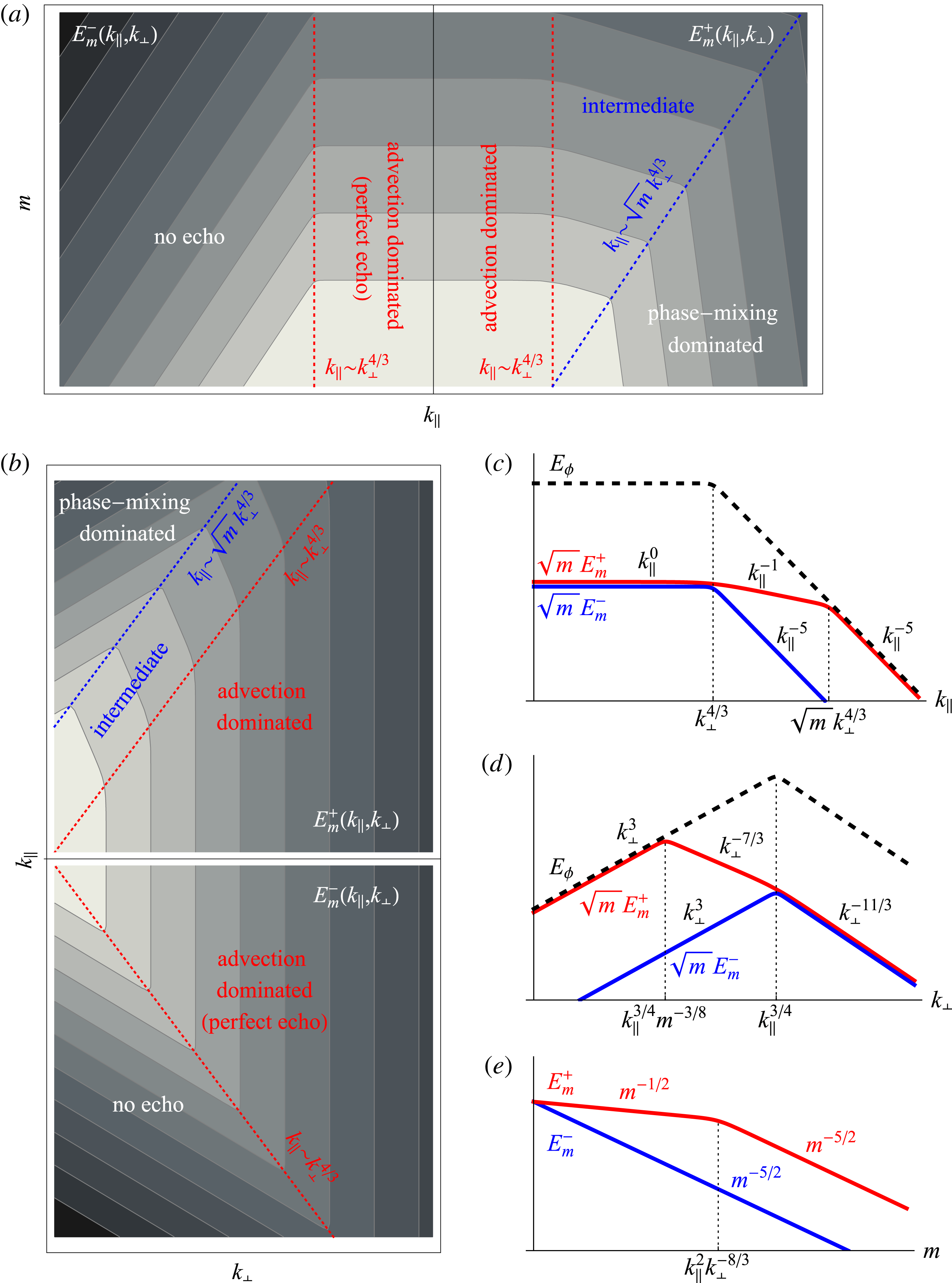
Figure 2. Spectra of higher Hermite moments, $E_{m}^{\pm }(k_{\Vert },k_{\bot })$
: (a) in the
$E_{m}^{\pm }(k_{\Vert },k_{\bot })$
: (a) in the $(k_{\Vert },m)$
plane at constant
$(k_{\Vert },m)$
plane at constant $k_{\bot }$
(
$k_{\bot }$
( $E_{m}^{+}$
and
$E_{m}^{+}$
and $E_{m}^{-}$
are shown in the right and left panels, respectively; in the left panel,
$E_{m}^{-}$
are shown in the right and left panels, respectively; in the left panel, $k_{\Vert }$
increases leftwards), (b) in the
$k_{\Vert }$
increases leftwards), (b) in the $(k_{\bot },k_{\Vert })$
plane at constant
$(k_{\bot },k_{\Vert })$
plane at constant $m$
(
$m$
( $E_{m}^{+}$
and
$E_{m}^{+}$
and $E_{m}^{-}$
are shown in the upper and lower panels, respectively; in the lower panel,
$E_{m}^{-}$
are shown in the upper and lower panels, respectively; in the lower panel, $k_{\Vert }$
increases downwards), (c) versus
$k_{\Vert }$
increases downwards), (c) versus $k_{\Vert }$
at constant
$k_{\Vert }$
at constant $k_{\bot }$
and
$k_{\bot }$
and $m$
, (d) versus
$m$
, (d) versus $k_{\bot }$
at constant
$k_{\bot }$
at constant $k_{\Vert }$
and
$k_{\Vert }$
and $m$
, (e) versus
$m$
, (e) versus $m$
at constant
$m$
at constant $k_{\Vert }$
and
$k_{\Vert }$
and $k_{\bot }$
(such that
$k_{\bot }$
(such that $k_{\Vert }>k_{\bot }^{4/3}$
, otherwise the spectra are
$k_{\Vert }>k_{\bot }^{4/3}$
, otherwise the spectra are $E_{m}^{\pm }\sim m^{-5/2}$
at all
$E_{m}^{\pm }\sim m^{-5/2}$
at all $m$
). All plots are logarithmic. The spectrum
$m$
). All plots are logarithmic. The spectrum $E_{{\it\varphi}}(k_{\Vert },k_{\bot })$
(see figure 1) is given in (c,d) as a dashed line, for reference. Free-energy flow through phase space as represented in (a,b) is described in § 5.2.
$E_{{\it\varphi}}(k_{\Vert },k_{\bot })$
(see figure 1) is given in (c,d) as a dashed line, for reference. Free-energy flow through phase space as represented in (a,b) is described in § 5.2.
Since we have fixed the value of the spectral exponent $a$
and since the spectra of
$a$
and since the spectra of ${\it\varphi}$
in the phase-mixing-dominated region, where this exponent applies, propagate to higher
${\it\varphi}$
in the phase-mixing-dominated region, where this exponent applies, propagate to higher $m$
’s, we now also have determined
$m$
’s, we now also have determined $E_{m}(k_{\Vert },k_{\bot })$
for
$E_{m}(k_{\Vert },k_{\bot })$
for $k_{\Vert }\gtrsim \sqrt{m}\,k_{\bot }^{r}$
: see (4.8).
$k_{\Vert }\gtrsim \sqrt{m}\,k_{\bot }^{r}$
: see (4.8).
Physically, the validity of the argument that led to the last set of results (see (4.15) onwards) hinges on our ability to produce phase-space spectra that are consistent with substantial cancellation of the phase-mixing flux at $k_{\Vert }\lesssim k_{\bot }^{r}$
and thus with the majority of the free energy residing in the low Hermite moments. Note that it is actually not controversial that the phase mixing should be negligible for
$k_{\Vert }\lesssim k_{\bot }^{r}$
and thus with the majority of the free energy residing in the low Hermite moments. Note that it is actually not controversial that the phase mixing should be negligible for $k_{\Vert }\ll k_{\bot }^{r}$
because this means the phase-mixing rate is low compared to the nonlinear-advection rate,
$k_{\Vert }\ll k_{\bot }^{r}$
because this means the phase-mixing rate is low compared to the nonlinear-advection rate, $k_{\Vert }v_{th}\ll k_{\bot }u_{\bot }$
, but, as we saw above, the energy is substantially dominated by the critical-balance curve
$k_{\Vert }v_{th}\ll k_{\bot }u_{\bot }$
, but, as we saw above, the energy is substantially dominated by the critical-balance curve $k_{\Vert }\sim k_{\bot }^{r}$
, where the two rates are comparable (recall our critique of the ‘fluid’ theory in § 2.4.4). In what follows, we shall build a case for the spectra that we have just derived – and so we will carefully avoid using the constant-flux argument (4.15) and keep all the scaling exponents general.
$k_{\Vert }\sim k_{\bot }^{r}$
, where the two rates are comparable (recall our critique of the ‘fluid’ theory in § 2.4.4). In what follows, we shall build a case for the spectra that we have just derived – and so we will carefully avoid using the constant-flux argument (4.15) and keep all the scaling exponents general.
4.3 Spectra of higher moments in the advection-dominated region
Let us now consider the higher Hermite moments, $m\gg 1$
. The condition for the phase-mixing rate to be negligible compared to the nonlinear-advection rate is the opposite of the condition (4.5):
$m\gg 1$
. The condition for the phase-mixing rate to be negligible compared to the nonlinear-advection rate is the opposite of the condition (4.5):
 $$\begin{eqnarray}\displaystyle k_{\Vert }v_{th}\ll \sqrt{m}k_{\bot }u_{\bot }\quad \Leftrightarrow \quad k_{\Vert }\ll \sqrt{m}k_{\bot }^{r} & & \displaystyle\end{eqnarray}$$
(i.e. the part of the phase space on the side of the phase-mixing threshold opposite to the phase-mixing-dominated region). In § 4.1, the phase-mixing threshold was derived by arguing that it represented the value of $s$
up to which the ‘
$s$
up to which the ‘ $+$
’ perturbations at some given
$+$
’ perturbations at some given $k_{\Vert }$
and
$k_{\Vert }$
and $k_{\bot }$
could propagate before being diverted to different wavenumbers by the nonlinear coupling. More generally and more formally, we may simply argue that, if, say, the
$k_{\bot }$
could propagate before being diverted to different wavenumbers by the nonlinear coupling. More generally and more formally, we may simply argue that, if, say, the $s$
dependence of
$s$
dependence of $\tilde{f}$
is a power law (which it must be; see appendix C), the size of the phase-mixing term in (3.12) can be estimated as
$\tilde{f}$
is a power law (which it must be; see appendix C), the size of the phase-mixing term in (3.12) can be estimated as ${\sim}(k_{\Vert }v_{th}/s)\tilde{f}$
, which is negligible compared to the nonlinear term if the condition (4.19) is satisfied.
${\sim}(k_{\Vert }v_{th}/s)\tilde{f}$
, which is negligible compared to the nonlinear term if the condition (4.19) is satisfied.
The advection-dominated region
 $$\begin{eqnarray}\displaystyle k_{\Vert }v_{th}\lesssim k_{\bot }u_{\bot }\quad \Leftrightarrow \quad k_{\Vert }\lesssim k_{\bot }^{r}, & & \displaystyle\end{eqnarray}$$
which, as we argued in § 4.2, contains most of the energy content of the low- $m$
Hermite moments (collectively represented by
$m$
Hermite moments (collectively represented by ${\it\varphi}$
) and, therefore, of the advecting velocity
${\it\varphi}$
) and, therefore, of the advecting velocity $\boldsymbol{u}_{\bot }$
, is well within the domain of validity of the condition (4.19), provided
$\boldsymbol{u}_{\bot }$
, is well within the domain of validity of the condition (4.19), provided $m\gg 1$
. Therefore, if we restrict our attention to the wavenumbers (4.20), we may neglect the phase-mixing term (second on the left-hand side) in (3.12) and thus deal with what is a purely ‘fluid’ equation for
$m\gg 1$
. Therefore, if we restrict our attention to the wavenumbers (4.20), we may neglect the phase-mixing term (second on the left-hand side) in (3.12) and thus deal with what is a purely ‘fluid’ equation for $\tilde{f}(s)$
at each
$\tilde{f}(s)$
at each $s$
. As we argued at the end of § 3.3, we can then have solutions satisfying
$s$
. As we argued at the end of § 3.3, we can then have solutions satisfying $\tilde{f}^{\ast }(k_{\Vert })=\tilde{f}(-k_{\Vert })$
, for which the ‘
$\tilde{f}^{\ast }(k_{\Vert })=\tilde{f}(-k_{\Vert })$
, for which the ‘ $+$
’ and ‘
$+$
’ and ‘ $-$
’ spectra are the same and the Hermite flux is zero (see (3.27)):
$-$
’ spectra are the same and the Hermite flux is zero (see (3.27)):
 $$\begin{eqnarray}\displaystyle E_{m}^{+}(k_{\Vert },k_{\bot })\approx E_{m}^{-}(k_{\Vert },k_{\bot }). & & \displaystyle\end{eqnarray}$$
Physically, this is because, in the advection-dominated region, the nonlinear coupling between positive and negative $k_{\Vert }$
mediated by the velocity field
$k_{\Vert }$
mediated by the velocity field $\boldsymbol{u}_{\bot }$
will be vigorous and fast – assuming, importantly, that interactions between
$\boldsymbol{u}_{\bot }$
will be vigorous and fast – assuming, importantly, that interactions between $\boldsymbol{u}_{\bot }$
and
$\boldsymbol{u}_{\bot }$
and $\tilde{f}$
are local in
$\tilde{f}$
are local in $k_{\Vert }$
and so, in the right-hand side of (3.12), the sum
$k_{\Vert }$
and so, in the right-hand side of (3.12), the sum $\sum _{p_{\Vert }}$
is dominated by wavenumber triads with
$\sum _{p_{\Vert }}$
is dominated by wavenumber triads with $p_{\Vert }\sim k_{\Vert }\sim k_{\Vert }-p_{\Vert }$
.
$p_{\Vert }\sim k_{\Vert }\sim k_{\Vert }-p_{\Vert }$
.
With the phase mixing neglected, the variance of $\tilde{f}$
is (approximately) conserved at each
$\tilde{f}$
is (approximately) conserved at each $s$
. The field
$s$
. The field $\tilde{f}(s)$
is nonlinearly cascaded to smaller scales (larger
$\tilde{f}(s)$
is nonlinearly cascaded to smaller scales (larger $k_{\bot }$
) by the advecting velocity
$k_{\bot }$
) by the advecting velocity $\boldsymbol{u}_{\bot }$
, so the standard constant-flux argument gives us
$\boldsymbol{u}_{\bot }$
, so the standard constant-flux argument gives us
 $$\begin{eqnarray}\displaystyle \tilde{f}^{2}(s)k_{\bot }u_{\bot }\sim \text{const}(s)\quad \Rightarrow \quad \tilde{f}^{2}(s)\propto k_{\bot }^{-r}\quad \Rightarrow \quad E_{m}^{\bot }(k_{\bot })\propto k_{\bot }^{-r-1}, & & \displaystyle\end{eqnarray}$$
where $E_{m}^{\bot }(k_{\bot })$
is the 1-D perpendicular spectrum of
$E_{m}^{\bot }(k_{\bot })$
is the 1-D perpendicular spectrum of $g_{m}$
. Note that the spectrum has an
$g_{m}$
. Note that the spectrum has an $m$
dependence, which cannot be determined via this argument.
$m$
dependence, which cannot be determined via this argument.
Since, in the advection-dominated region (4.20), the parallel-communication times are long compared to the nonlinear-decorrelation times, the perturbations can be expected to have a white-noise spectrum in $k_{\Vert }$
. Therefore, we can write their 2-D spectrum as follows
$k_{\Vert }$
. Therefore, we can write their 2-D spectrum as follows
 $$\begin{eqnarray}\displaystyle E_{m}(k_{\Vert },k_{\bot })\sim E_{m}^{\pm }(k_{\Vert },k_{\bot })\sim \frac{k_{\Vert }^{0}k_{\bot }^{-d}}{m^{{\it\sigma}}},\quad k_{\Vert }\lesssim k_{\bot }^{r}, & & \displaystyle\end{eqnarray}$$
where we have allowed for an as yet unknown scaling with $m$
. The
$m$
. The $k_{\bot }$
-scaling exponent
$k_{\bot }$
-scaling exponent $d$
can be determined via the requirement that (4.23) be consistent with (4.22): assuming that, for any given
$d$
can be determined via the requirement that (4.23) be consistent with (4.22): assuming that, for any given $k_{\bot }$
, the region
$k_{\bot }$
, the region $k_{\Vert }\lesssim k_{\bot }^{r}$
contains most of the energy,Footnote
18
$k_{\Vert }\lesssim k_{\bot }^{r}$
contains most of the energy,Footnote
18
 $$\begin{eqnarray}\displaystyle E_{m}^{\bot }(k_{\bot })=\int \text{d}k_{\Vert }E_{m}(k_{\Vert },k_{\bot })\sim \int _{0}^{k_{\bot }^{r}}\text{d}k_{\Vert }\frac{k_{\Vert }^{0}k_{\bot }^{-d}}{m^{{\it\sigma}}}\propto k_{\bot }^{-(d-r)}\quad \Rightarrow \quad d=1+2r. & & \displaystyle\end{eqnarray}$$
Since, as we have argued here, the Hermite flux is (approximately) zero in this region of wavenumber space for all higher $m$
’s, there can be very little net free-energy flow out of low
$m$
’s, there can be very little net free-energy flow out of low $m$
’s – and so, in retrospect, we were justified in assuming in § 4.2 that the energy of the low-
$m$
’s – and so, in retrospect, we were justified in assuming in § 4.2 that the energy of the low- $m$
moments was conserved and so a constant-flux argument (4.15) could be used to deduce the scaling of
$m$
moments was conserved and so a constant-flux argument (4.15) could be used to deduce the scaling of ${\it\varphi}$
. This allows us to adopt the scaling exponents (4.16) (which we have thus far avoided using), in particular,
${\it\varphi}$
. This allows us to adopt the scaling exponents (4.16) (which we have thus far avoided using), in particular, $r=4/3$
, and so, using (4.24), the free-energy spectrum is (see figure 2 for illustration)
$r=4/3$
, and so, using (4.24), the free-energy spectrum is (see figure 2 for illustration)
 $$\begin{eqnarray}\displaystyle E_{m}^{\pm }(k_{\Vert },k_{\bot })\sim \frac{k_{\Vert }^{0}k_{\bot }^{-11/3}}{m^{{\it\sigma}}},\quad k_{\Vert }\lesssim k_{\bot }^{4/3}. & & \displaystyle\end{eqnarray}$$
Unsurprisingly, there is continuity between the scalings of $E_{m}^{\pm }$
and the scaling of
$E_{m}^{\pm }$
and the scaling of $E_{{\it\varphi}}$
. The scaling exponent
$E_{{\it\varphi}}$
. The scaling exponent ${\it\sigma}$
will be found in § 4.4.1.
${\it\sigma}$
will be found in § 4.4.1.
Before moving on to complete our scaling theory, we note that jumping to the result (4.25) already in this section was borne of pure impatience: we will discover in § 4.4 that, in fact, it is possible to determine the scaling exponent $d$
without relying on the as yet perhaps somewhat unconvincing claim that a constant-flux argument is legitimate for
$d$
without relying on the as yet perhaps somewhat unconvincing claim that a constant-flux argument is legitimate for ${\it\varphi}$
despite the phase mixing being notionally not small along the critical-balance curve
${\it\varphi}$
despite the phase mixing being notionally not small along the critical-balance curve $k_{\Vert }\sim k_{\bot }^{r}$
.
$k_{\Vert }\sim k_{\bot }^{r}$
.
4.4 Intermediate region and matching conditions
We now have the form of the free-energy spectra in two regions, $k_{\Vert }\gtrsim \sqrt{m}\,k_{\bot }^{r}$
(phase-mixing dominated, very little free energy, see (4.8)) and
$k_{\Vert }\gtrsim \sqrt{m}\,k_{\bot }^{r}$
(phase-mixing dominated, very little free energy, see (4.8)) and $k_{\Vert }\lesssim k_{\bot }^{r}$
(advection-dominated cascade, contains most of the free energy, see (4.25)). It remains to determine the free-energy spectrum in the intermediate region between these two:
$k_{\Vert }\lesssim k_{\bot }^{r}$
(advection-dominated cascade, contains most of the free energy, see (4.25)). It remains to determine the free-energy spectrum in the intermediate region between these two:
 $$\begin{eqnarray}\displaystyle E_{m}^{+}(k_{\Vert },k_{\bot })\sim \frac{k_{\Vert }^{-a^{\prime }}k_{\bot }^{-d^{\prime }}}{m^{{\it\sigma}^{\prime }}},\quad k_{\bot }^{r}\lesssim k_{\Vert }\lesssim \sqrt{m}\,k_{\bot }^{r} & & \displaystyle\end{eqnarray}$$
(the following argument will only apply to the ‘ $+$
’ modes; both the reasons for this and the way to determine the spectrum of the ‘
$+$
’ modes; both the reasons for this and the way to determine the spectrum of the ‘ $-$
’ modes will be explained in § 4.5).
$-$
’ modes will be explained in § 4.5).
We have three new scaling exponents, but we also have the requirement to match (4.26) with (4.8) and (4.23) along the boundaries of the intermediate region. This gives us four relations
 $$\begin{eqnarray}\displaystyle {\it\sigma}^{\prime }={\it\sigma},\quad d^{\prime }+a^{\prime }r=d,\quad d^{\prime }+a^{\prime }r=ar-3,\quad a^{\prime }+2{\it\sigma}^{\prime }=1+a, & & \displaystyle\end{eqnarray}$$
which we rearrange so:
 $$\begin{eqnarray}\displaystyle a^{\prime }=\frac{d-d^{\prime }}{r},\quad d=ar-3,\quad {\it\sigma}={\it\sigma}^{\prime }=\frac{3+r+d^{\prime }}{2r}. & & \displaystyle\end{eqnarray}$$
Let us combine these with two equally uncontroversial (i.e. requiring no leaps of physical intuition) matching and consistency relations from § 4.2: (4.11) and (4.13), which we can rewrite as
 $$\begin{eqnarray}\displaystyle a=\frac{8-r}{r},\quad c=5-r. & & \displaystyle\end{eqnarray}$$
The second of equations (4.28) then gives
 $$\begin{eqnarray}\displaystyle d=5-r=c. & & \displaystyle\end{eqnarray}$$
Thus, the perpendicular scalings of $E_{m}^{\pm }$
and
$E_{m}^{\pm }$
and $E_{{\it\varphi}}$
must be the same in the advection-dominated region
$E_{{\it\varphi}}$
must be the same in the advection-dominated region $k_{\Vert }\lesssim k_{\bot }^{r}$
. If we bring in (4.24), i.e. the constant-flux argument (4.22), we get immediately
$k_{\Vert }\lesssim k_{\bot }^{r}$
. If we bring in (4.24), i.e. the constant-flux argument (4.22), we get immediately
 $$\begin{eqnarray}\displaystyle r={\textstyle \frac{4}{3}},\quad d=c={\textstyle \frac{11}{3}},\quad a=5. & & \displaystyle\end{eqnarray}$$
These are the same as the exponents (4.16), except the need for the ‘fluid’ constant-flux argument (4.15) for ${\it\varphi}$
has now been obviated by the combination of a more solid phase-space argument (4.22) and a number of inevitable consistency relations. Equations (4.28) will give us
${\it\varphi}$
has now been obviated by the combination of a more solid phase-space argument (4.22) and a number of inevitable consistency relations. Equations (4.28) will give us $a^{\prime }$
,
$a^{\prime }$
, ${\it\sigma}^{\prime }$
and
${\it\sigma}^{\prime }$
and ${\it\sigma}$
if we know
${\it\sigma}$
if we know $d^{\prime }$
. In order to determine the latter, we must now consider why physics in the intermediate phase-space region
$d^{\prime }$
. In order to determine the latter, we must now consider why physics in the intermediate phase-space region $k_{\bot }^{r}\lesssim k_{\Vert }\lesssim \sqrt{m}\,k_{\bot }^{r}$
should be at all different from what happens in the advection-dominated region
$k_{\bot }^{r}\lesssim k_{\Vert }\lesssim \sqrt{m}\,k_{\bot }^{r}$
should be at all different from what happens in the advection-dominated region $k_{\Vert }\lesssim k_{\bot }^{r}$
considered in § 4.3 (and so why
$k_{\Vert }\lesssim k_{\bot }^{r}$
considered in § 4.3 (and so why $d^{\prime }\neq d$
).
$d^{\prime }\neq d$
).
4.4.1 Spectra in the intermediate region
Except at the phase-mixing threshold $k_{\Vert }\sim \sqrt{m}\,k_{\bot }^{r}$
(which is considered with more care in appendix C), phase mixing in the intermediate region is dominated by nonlinear advection. However, interactions between
$k_{\Vert }\sim \sqrt{m}\,k_{\bot }^{r}$
(which is considered with more care in appendix C), phase mixing in the intermediate region is dominated by nonlinear advection. However, interactions between $\boldsymbol{u}_{\bot }$
and
$\boldsymbol{u}_{\bot }$
and $\tilde{f}$
cannot, unlike in the advection-dominated region discussed in § 4.3, be local in
$\tilde{f}$
cannot, unlike in the advection-dominated region discussed in § 4.3, be local in $k_{\Vert }$
. Indeed, we know from § 4.2 that there is very little energy left in
$k_{\Vert }$
. Indeed, we know from § 4.2 that there is very little energy left in $\boldsymbol{u}_{\bot }$
at
$\boldsymbol{u}_{\bot }$
at $k_{\Vert }\gg k_{\bot }^{r}$
. Assuming interactions to be local in
$k_{\Vert }\gg k_{\bot }^{r}$
. Assuming interactions to be local in $k_{\bot }$
, the wavenumber sum in the right-hand side of (3.12) will be dominated by
$k_{\bot }$
, the wavenumber sum in the right-hand side of (3.12) will be dominated by $p_{\Vert }\lesssim k_{\bot }^{r}$
(see appendix B for a careful analysis of the possible non-local interactions in the intermediate region). If
$p_{\Vert }\lesssim k_{\bot }^{r}$
(see appendix B for a careful analysis of the possible non-local interactions in the intermediate region). If $k_{\Vert }\gg k_{\bot }^{r}$
, then
$k_{\Vert }\gg k_{\bot }^{r}$
, then $p_{\Vert }\ll k_{\Vert }$
,
$p_{\Vert }\ll k_{\Vert }$
, $\tilde{f}(k_{\Vert }-p_{\Vert })\approx \tilde{f}(k_{\Vert })$
, and so (3.12) now describes the advection of
$\tilde{f}(k_{\Vert }-p_{\Vert })\approx \tilde{f}(k_{\Vert })$
, and so (3.12) now describes the advection of $\tilde{f}(s,k_{\Vert })$
by an essentially 2-D velocity field (its parallel scale is much longer than that of
$\tilde{f}(s,k_{\Vert })$
by an essentially 2-D velocity field (its parallel scale is much longer than that of $\tilde{f}$
), with both
$\tilde{f}$
), with both $s$
and
$s$
and $k_{\Vert }$
appearing as implicit parameters. This means that the variance of
$k_{\Vert }$
appearing as implicit parameters. This means that the variance of $\tilde{f}$
will be conserved for each individual
$\tilde{f}$
will be conserved for each individual $s$
and
$s$
and $k_{\Vert }$
Footnote
19
– and this in turn, by yet another constant-flux-in-
$k_{\Vert }$
Footnote
19
– and this in turn, by yet another constant-flux-in- $k_{\bot }$
argument, implies
$k_{\bot }$
argument, implies
 $$\begin{eqnarray}\displaystyle \tilde{f}^{2}(s,k_{\Vert })k_{\bot }u_{\bot }\sim \text{const}\;(s,k_{\Vert })\quad \Rightarrow \quad \tilde{f}^{2}(s,k_{\Vert })\propto k_{\bot }^{-r}\quad \Rightarrow \quad E_{m}(k_{\Vert },k_{\bot })\propto k_{\bot }^{-r-1}.\quad & & \displaystyle\end{eqnarray}$$
This scaling is of the 2-D spectrum, not of the 1-D perpendicular one, because $k_{\Vert }$
is a fixed parameter rather than a variable over which there can be any nonlinear coupling. Comparing (4.26) and (4.32), we read off
$k_{\Vert }$
is a fixed parameter rather than a variable over which there can be any nonlinear coupling. Comparing (4.26) and (4.32), we read off $d^{\prime }$
and hence, with the aid of the first and third equations (4.28), complete the determination of all scaling exponents:
$d^{\prime }$
and hence, with the aid of the first and third equations (4.28), complete the determination of all scaling exponents:
 $$\begin{eqnarray}\displaystyle d^{\prime }=r+1={\textstyle \frac{7}{3}},\quad a^{\prime }=1,\quad {\it\sigma}^{\prime }={\it\sigma}={\textstyle \frac{5}{2}}. & & \displaystyle\end{eqnarray}$$
Thus, the free-energy spectrum in the intermediate region is
 $$\begin{eqnarray}\displaystyle E_{m}^{+}(k_{\Vert },k_{\bot })\sim \frac{k_{\Vert }^{-1}k_{\bot }^{-7/3}}{m^{5/2}},\quad k_{\bot }^{4/3}\lesssim k_{\Vert }\lesssim \sqrt{m}\,k_{\bot }^{4/3}, & & \displaystyle\end{eqnarray}$$
sketched in figure 2. The spectrum of the ‘ $-$
’ modes will be discussed in § 4.5.
$-$
’ modes will be discussed in § 4.5.
4.4.2 1-D spectra
In the run up to (4.24), we assumed that integrating the 2-D spectrum $E_{m}(k_{\Vert },k_{\bot })$
with respect to
$E_{m}(k_{\Vert },k_{\bot })$
with respect to $k_{\Vert }$
over the advection-dominated region
$k_{\Vert }$
over the advection-dominated region $k_{\Vert }\lesssim k_{\bot }^{r}$
captures most of the free energy contained in any fixed
$k_{\Vert }\lesssim k_{\bot }^{r}$
captures most of the free energy contained in any fixed $k_{\bot }$
. Now in possession of (4.34), we see that this is not entirely correct: in fact, using now both (4.25) and (4.34), we find the 1-D perpendicular spectrum to be
$k_{\bot }$
. Now in possession of (4.34), we see that this is not entirely correct: in fact, using now both (4.25) and (4.34), we find the 1-D perpendicular spectrum to be
 $$\begin{eqnarray}\displaystyle E_{m}^{\bot +}(k_{\bot }) & = & \displaystyle \int \text{d}k_{\Vert }E_{m}^{+}(k_{\Vert },k_{\bot })\nonumber\\ \displaystyle & {\sim} & \displaystyle \int _{0}^{k_{\bot }^{4/3}}\text{d}k_{\Vert }\frac{k_{\Vert }^{0}k_{\bot }^{-11/3}}{m^{5/2}}+\int _{k_{\bot }^{4/3}}^{\sqrt{m}k_{\bot }^{4/3}}\text{d}k_{\Vert }\frac{k_{\Vert }^{-1}k_{\bot }^{-7/3}}{m^{5/2}}\sim \frac{k_{\bot }^{-7/3}}{m^{5/2}}(1+\ln \sqrt{m}).\end{eqnarray}$$
So there is logarithmically more free energy in the intermediate region, but this does not affect the $k_{\bot }$
scaling, which is what we were after in (4.24), so the derivation in § 4.3 survives.
$k_{\bot }$
scaling, which is what we were after in (4.24), so the derivation in § 4.3 survives.
For completeness, let us also calculate the 1-D parallel spectrum. Integration over $k_{\bot }$
is dominated by the wavenumbers around the phase-mixing threshold
$k_{\bot }$
is dominated by the wavenumbers around the phase-mixing threshold $k_{\bot }\sim (k_{\Vert }/\sqrt{m})^{3/4}$
, so
$k_{\bot }\sim (k_{\Vert }/\sqrt{m})^{3/4}$
, so
 $$\begin{eqnarray}\displaystyle E_{m}^{\Vert +}(k_{\Vert }) & = & \displaystyle \int \text{d}k_{\bot }\,E_{m}^{+}(k_{\Vert },k_{\bot })\nonumber\\ \displaystyle & {\sim} & \displaystyle \int _{0}^{(k_{\Vert }/\sqrt{m})^{3/4}}\text{d}k_{\bot }\frac{k_{\bot }^{3}k_{\Vert }^{-5}}{\sqrt{m}}+\int _{(k_{\Vert }/\sqrt{m})^{3/4}}^{k_{\Vert }^{3/4}}\text{d}k_{\bot }\frac{k_{\Vert }^{-1}k_{\bot }^{-7/3}}{m^{5/2}}\sim \frac{k_{\Vert }^{-2}}{m^{2}}.\end{eqnarray}$$
Note that this $m^{-2}$
scaling appears to be in decent agreement with the Hermite-space spectra reported by Hatch et al. (Reference Hatch, Jenko, Bañón Navarro and Bratanov2013, Reference Hatch, Jenko, Bratanov and Bañón Navarro2014).
$m^{-2}$
scaling appears to be in decent agreement with the Hermite-space spectra reported by Hatch et al. (Reference Hatch, Jenko, Bañón Navarro and Bratanov2013, Reference Hatch, Jenko, Bratanov and Bañón Navarro2014).
A perceptive reader might be feeling a growing resentment over our use of the spectrum (4.34) at wavenumbers around the phase-mixing threshold $k_{\Vert }\sim \sqrt{m}\,k_{\bot }^{4/3}$
, even though, technically speaking, we have only justified (4.34) in the region
$k_{\Vert }\sim \sqrt{m}\,k_{\bot }^{4/3}$
, even though, technically speaking, we have only justified (4.34) in the region $k_{\bot }^{4/3}\lesssim k_{\Vert }\ll \sqrt{m}k_{\bot }^{4/3}$
, seeing that at
$k_{\bot }^{4/3}\lesssim k_{\Vert }\ll \sqrt{m}k_{\bot }^{4/3}$
, seeing that at $k_{\Vert }\sim \sqrt{m}k_{\bot }^{4/3}$
, phase mixing cannot be neglected compared to the nonlinear advection. In appendix C, we show that it nevertheless makes sense simply to match the spectrum (4.26) to the phase-mixing-dominated spectrum (4.8) along the phase-mixing threshold.
$k_{\Vert }\sim \sqrt{m}k_{\bot }^{4/3}$
, phase mixing cannot be neglected compared to the nonlinear advection. In appendix C, we show that it nevertheless makes sense simply to match the spectrum (4.26) to the phase-mixing-dominated spectrum (4.8) along the phase-mixing threshold.
4.5 Anti-phase-mixing spectra
The arguments about the intermediate-region spectra presented in § 4.4 only apply to the spectrum of the ‘ $+$
’ modes. Since the advection velocity is effectively 2-D in the intermediate region (see § 4.4.1), there is no coupling between different parallel wavenumbers and so no echo effect. Thus, if, as we argued in § 4.3,
$+$
’ modes. Since the advection velocity is effectively 2-D in the intermediate region (see § 4.4.1), there is no coupling between different parallel wavenumbers and so no echo effect. Thus, if, as we argued in § 4.3, $E_{m}^{-}\approx E_{m}^{+}\propto k_{\bot }^{-d}$
in the advection-dominated region,
$E_{m}^{-}\approx E_{m}^{+}\propto k_{\bot }^{-d}$
in the advection-dominated region, $k_{\bot }\gtrsim k_{\Vert }^{1/r}$
, due to vigorous coupling between parallel wavenumbers, and
$k_{\bot }\gtrsim k_{\Vert }^{1/r}$
, due to vigorous coupling between parallel wavenumbers, and $E_{m}^{-}\ll E_{m}^{+}$
in the intermediate and phase-mixing-dominated region,
$E_{m}^{-}\ll E_{m}^{+}$
in the intermediate and phase-mixing-dominated region, $k_{\bot }\ll k_{\Vert }^{1/r}$
, due to absence of any such coupling, we must expect that the energy-containing wavenumbers for the ‘
$k_{\bot }\ll k_{\Vert }^{1/r}$
, due to absence of any such coupling, we must expect that the energy-containing wavenumbers for the ‘ $-$
’ modes are ones along the critical-balance curve
$-$
’ modes are ones along the critical-balance curve $k_{\bot }\sim k_{\Vert }^{1/r}$
.
$k_{\bot }\sim k_{\Vert }^{1/r}$
.
The $k_{\bot }\rightarrow 0$
asymptotic behaviour of the ‘
$k_{\bot }\rightarrow 0$
asymptotic behaviour of the ‘ $-$
’ spectrum must be the same as for any other field,
$-$
’ spectrum must be the same as for any other field, $E_{m}^{-}\propto k_{\bot }^{3}$
, because the reasons for it are purely kinematic (appendix A). Thus, we posit
$E_{m}^{-}\propto k_{\bot }^{3}$
, because the reasons for it are purely kinematic (appendix A). Thus, we posit
 $$\begin{eqnarray}\displaystyle E_{m}^{-}(k_{\Vert },k_{\bot })\sim \frac{k_{\bot }^{3}k_{\Vert }^{-a^{\prime \prime }}}{m^{{\it\sigma}^{\prime \prime }}},\quad k_{\Vert }\gtrsim k_{\bot }^{r} & & \displaystyle\end{eqnarray}$$
and impose matching conditions between this spectrum and (4.23) at $k_{\Vert }\sim k_{\bot }^{r}$
:
$k_{\Vert }\sim k_{\bot }^{r}$
:
 $$\begin{eqnarray}\displaystyle a^{\prime \prime }=\frac{d+3}{r}=5,\quad {\it\sigma}^{\prime \prime }={\it\sigma}=\frac{5}{2}. & & \displaystyle\end{eqnarray}$$
This completes the determination of the phase-space spectra of the anti-phase-mixing component of the free energy:
 $$\begin{eqnarray}\displaystyle E_{m}^{-}(k_{\Vert },k_{\bot })\sim \frac{1}{m^{5/2}}\left\{\begin{array}{@{}ll@{}}\displaystyle k_{\bot }^{3}k_{\Vert }^{-5}, & \text{if }k_{\Vert }\gtrsim k_{\bot }^{4/3},\\ \displaystyle k_{\Vert }^{0}k_{\bot }^{-11/3}, & \text{if }k_{\Vert }\lesssim k_{\bot }^{4/3}.\end{array}\right. & & \displaystyle\end{eqnarray}$$
Figure 2 shows these and illustrates their relationship to other spectra derived above.
The 1-D spectra that follow from (4.39) are
 $$\begin{eqnarray}\displaystyle & \displaystyle E_{m}^{\bot -}(k_{\bot })=\int \text{d}k_{\Vert }E_{m}^{-}(k_{\Vert },k_{\bot })\sim \frac{k_{\bot }^{-7/3}}{m^{5/2}}, & \displaystyle\end{eqnarray}$$
 $$\begin{eqnarray}\displaystyle & \displaystyle E_{m}^{\Vert -}(k_{\Vert })=\int \text{d}k_{\bot }E_{m}^{-}(k_{\Vert },k_{\bot })\sim \frac{k_{\Vert }^{-2}}{m^{5/2}}. & \displaystyle\end{eqnarray}$$ $m$
, to the ‘
$m$
, to the ‘ $+$
’-mode spectra (4.35) and (4.36).
$+$
’-mode spectra (4.35) and (4.36).
4.6 Effect of collisions
4.6.1 Collisional cutoff for phase-mixing modes
In the phase-mixing-dominated regime (§ 4.1), the collisional cutoff is set, in the same way as in the linear theory (§ 2.5), by the competition between the phase-mixing rate ${\sim}k_{\Vert }v_{th}/\sqrt{m}$
and the collision rate
${\sim}k_{\Vert }v_{th}/\sqrt{m}$
and the collision rate ${\sim}{\it\nu}m$
. The perturbations are collisionally damped if
${\sim}{\it\nu}m$
. The perturbations are collisionally damped if
 $$\begin{eqnarray}\displaystyle {\it\nu}m\gtrsim \frac{k_{\Vert }v_{th}}{\sqrt{m}}\gtrsim k_{\bot }u_{\bot }\quad \Leftrightarrow \quad m\gtrsim \left(\frac{k_{\Vert }}{{\it\nu}}\right)^{2/3},\quad k_{\Vert }\gtrsim \frac{k_{\bot }^{2}}{\sqrt{{\it\nu}}}, & & \displaystyle\end{eqnarray}$$
giving a cutoff in Hermite space (cf. (2.59)).Footnote 20 In both the intermediate (§ 4.4) and advection-dominated (§ 4.3) regimes, the relevant comparison is between the collision rate and the nonlinear-advection rate:
 $$\begin{eqnarray}\displaystyle {\it\nu}m\gtrsim k_{\bot }u_{\bot }\gtrsim \frac{k_{\Vert }v_{th}}{\sqrt{m}}\quad \Leftrightarrow \quad m\gtrsim \frac{k_{\bot }^{4/3}}{{\it\nu}},\quad k_{\Vert }\lesssim \frac{k_{\bot }^{2}}{\sqrt{{\it\nu}}}. & & \displaystyle\end{eqnarray}$$
These cutoffs are sketched in figure 3.
At a fixed $m$
, the above relations imply that there is an infrared collisional cutoff in the
$m$
, the above relations imply that there is an infrared collisional cutoff in the $(k_{\Vert },k_{\bot })$
space: perturbations are damped if
$(k_{\Vert },k_{\bot })$
space: perturbations are damped if
 $$\begin{eqnarray}\displaystyle k_{\Vert }\lesssim {\it\nu}m^{3/2},\quad k_{\bot }\lesssim ({\it\nu}m)^{3/4}. & & \displaystyle\end{eqnarray}$$
These cutoffs will not, of course, be relevant in comparison with the outer scales ( $k_{\Vert 0}$
and
$k_{\Vert 0}$
and $k_{\bot 0}$
; see § 2.4.1) except at high enough
$k_{\bot 0}$
; see § 2.4.1) except at high enough $m$
or if the collision frequency approaches the characteristic phase-mixing and nonlinear-advection rates at the outer scale. In the latter case, one expects some amount of free energy to drain via collisional dissipation around the outer scale, petering out at larger
$m$
or if the collision frequency approaches the characteristic phase-mixing and nonlinear-advection rates at the outer scale. In the latter case, one expects some amount of free energy to drain via collisional dissipation around the outer scale, petering out at larger $(k_{\Vert },k_{\bot })$
, where the collisionless physics asserts itself (cf. Hatch et al.
Reference Hatch, Terry, Jenko, Merz and Nevins2011a
,Reference Hatch, Terry, Jenko, Merz, Pueschel, Nevins and Wang
b
, Reference Hatch, Jenko, Bañón Navarro and Bratanov2013, Reference Hatch, Jenko, Bratanov and Bañón Navarro2014).
$(k_{\Vert },k_{\bot })$
, where the collisionless physics asserts itself (cf. Hatch et al.
Reference Hatch, Terry, Jenko, Merz and Nevins2011a
,Reference Hatch, Terry, Jenko, Merz, Pueschel, Nevins and Wang
b
, Reference Hatch, Jenko, Bañón Navarro and Bratanov2013, Reference Hatch, Jenko, Bratanov and Bañón Navarro2014).

Figure 3. Partition of phase space, viz., $(k_{\Vert },m)$
plane at fixed
$(k_{\Vert },m)$
plane at fixed $k_{\bot }$
, showing the collision-dominated region, cf. figure 2(a). All axes are logarithmic (in the left panel,
$k_{\bot }$
, showing the collision-dominated region, cf. figure 2(a). All axes are logarithmic (in the left panel, $k_{\Vert }$
increases leftwards).
$k_{\Vert }$
increases leftwards).
4.6.2 Collisional cutoff for anti-phase-mixing modes
The collisional cutoff (4.43) on the free-energy spectrum of the ‘ $+$
’ modes in the advection-dominated regime must extend to the ‘
$+$
’ modes in the advection-dominated regime must extend to the ‘ $-$
’ (anti-phase-mixing) modes because nonlinear coupling is the only source of the latter (see § 4.3). But the anti-phase-mixing modes propagate from high to low
$-$
’ (anti-phase-mixing) modes because nonlinear coupling is the only source of the latter (see § 4.3). But the anti-phase-mixing modes propagate from high to low $m$
and so a zero ‘boundary condition’ at high
$m$
and so a zero ‘boundary condition’ at high $m$
will be imprinted onto a region of phase space at lower
$m$
will be imprinted onto a region of phase space at lower $m$
’s. To wit, arguing analogously to § 4.1 and considering now
$m$
’s. To wit, arguing analogously to § 4.1 and considering now $k_{\Vert }<0$
in (3.12), we note that anti-phase-mixing modes propagate along the characteristics
$k_{\Vert }<0$
in (3.12), we note that anti-phase-mixing modes propagate along the characteristics
 $$\begin{eqnarray}\displaystyle s=-\frac{|k_{\Vert }|v_{th}}{\sqrt{2}}t+s_{0}, & & \displaystyle\end{eqnarray}$$
where $s_{0}$
is a constant. Whatever anti-phase-mixing spectrum exists at
$s_{0}$
is a constant. Whatever anti-phase-mixing spectrum exists at $s=s_{0}$
, it will be replicated over all
$s=s_{0}$
, it will be replicated over all $s$
satisfying (4.45) for times shorter than the nonlinear time,
$s$
satisfying (4.45) for times shorter than the nonlinear time, $t\lesssim {\it\tau}_{nl}\sim (k_{\bot }u_{\bot })^{-1}\sim k_{\bot }^{4/3}$
. Assuming that
$t\lesssim {\it\tau}_{nl}\sim (k_{\bot }u_{\bot })^{-1}\sim k_{\bot }^{4/3}$
. Assuming that $E_{m}^{-}$
is cut off for
$E_{m}^{-}$
is cut off for $s\gtrsim s_{c}=k_{\bot }^{2/3}/\sqrt{{\it\nu}}$
(see (4.43)) and letting
$s\gtrsim s_{c}=k_{\bot }^{2/3}/\sqrt{{\it\nu}}$
(see (4.43)) and letting $s_{0}=s_{c}$
, we conclude that
$s_{0}=s_{c}$
, we conclude that $E_{m}^{-}$
must also be cut off for
$E_{m}^{-}$
must also be cut off for
 $$\begin{eqnarray}\displaystyle s\gtrsim s_{c}-\frac{|k_{\Vert }|v_{th}}{k_{\bot }u_{\bot }}\quad \Leftrightarrow \quad \sqrt{m}\gtrsim \sqrt{m_{c}}-\frac{|k_{\Vert }|}{k_{\bot }^{4/3}},\quad m_{c}=\frac{k_{\bot }^{4/3}}{{\it\nu}}. & & \displaystyle\end{eqnarray}$$
This implies, in particular, that there is no anti-phase-mixing energy at any $m$
’s for wavenumbers satisfying
$m$
’s for wavenumbers satisfying
 $$\begin{eqnarray}\displaystyle |k_{\Vert }|\gtrsim \frac{k_{\bot }^{2}}{\sqrt{{\it\nu}}}. & & \displaystyle\end{eqnarray}$$
The collision-dominated region of the phase space is sketched in figure 3.
Whereas the collisional cutoff is safely removed to infinite $m$
in the limit
$m$
in the limit ${\it\nu}\rightarrow 0$
, in systems with only moderately low collision frequency, one should expect to see a finite reduction in the anti-phase-mixing flux at higher
${\it\nu}\rightarrow 0$
, in systems with only moderately low collision frequency, one should expect to see a finite reduction in the anti-phase-mixing flux at higher $m$
’s, as per (4.46).
$m$
’s, as per (4.46).
4.7 Total free energy and dissipation
In the linear problem, where all energy injected into the system had to be removed by Landau damping (meaning phase mixing followed by collisional dissipation at high $m$
), the free energy stored in phase space in a steady state had to diverge with vanishing collisionality (see (2.61)) in order for the dissipation to remain finite (see (2.60)). In the nonlinear situation with which we are now preoccupied, the Hermite spectra are steep power laws and so the free energy will be finite and collisional dissipation vanish, with all of the injected energy having to be removed via dissipation at small spatial scales (sub-Larmor and so outside the regime of validity of this theory).
$m$
), the free energy stored in phase space in a steady state had to diverge with vanishing collisionality (see (2.61)) in order for the dissipation to remain finite (see (2.60)). In the nonlinear situation with which we are now preoccupied, the Hermite spectra are steep power laws and so the free energy will be finite and collisional dissipation vanish, with all of the injected energy having to be removed via dissipation at small spatial scales (sub-Larmor and so outside the regime of validity of this theory).
To demonstrate this a little more quantitatively, let us repeat the calculation of the 1-D parallel spectrum (4.36), but now, in integrating the 2-D spectrum over $k_{\bot }$
, we assume that there is no free energy at perpendicular wavenumbers below the collisional cutoff
$k_{\bot }$
, we assume that there is no free energy at perpendicular wavenumbers below the collisional cutoff $k_{\bot }\sim ({\it\nu}m)^{3/4}$
(see (4.44)). The following three cases correspond to the collisional cutoff falling into the phase-mixing-dominated, intermediate and advection-dominated regions, respectively:
$k_{\bot }\sim ({\it\nu}m)^{3/4}$
(see (4.44)). The following three cases correspond to the collisional cutoff falling into the phase-mixing-dominated, intermediate and advection-dominated regions, respectively:
 $$\begin{eqnarray}\displaystyle E_{m}^{\Vert +}(k_{\Vert })\sim \left\{\begin{array}{@{}ll@{}}\displaystyle \frac{k_{\Vert }^{-2}}{m^{2}} & \text{if }m\lesssim \left(\displaystyle \frac{k_{\Vert }}{{\it\nu}}\right)^{2/3}\sim m_{c},\\ \displaystyle \frac{k_{\Vert }^{-1}}{{\it\nu}m^{7/2}} & \text{if }\left(\displaystyle \frac{k_{\Vert }}{{\it\nu}}\right)^{2/3}\lesssim m\lesssim \displaystyle \frac{k_{\Vert }}{{\it\nu}},\\ \displaystyle \frac{k_{\Vert }^{0}}{{\it\nu}^{2}m^{9/2}} & \text{if }m\gtrsim \displaystyle \frac{k_{\Vert }}{{\it\nu}}.\end{array}\right. & & \displaystyle\end{eqnarray}$$
Note that the last two cases are only relevant at very high $m$
(because
$m$
(because $k_{\Vert }\geqslant k_{\Vert 0}\sim 1$
, the outer scale in our units). Now integrating these spectra over
$k_{\Vert }\geqslant k_{\Vert 0}\sim 1$
, the outer scale in our units). Now integrating these spectra over $m$
, we find that the total free energy in a given
$m$
, we find that the total free energy in a given $k_{\Vert }$
is completely dominated by low
$k_{\Vert }$
is completely dominated by low $m$
’s:
$m$
’s:
 $$\begin{eqnarray}\displaystyle W(k_{\Vert })\sim \int _{{\sim}1}^{\infty }\text{d}mE_{m}^{\Vert +}(k_{\Vert })\sim k_{\Vert }^{-2}. & & \displaystyle\end{eqnarray}$$
The total collisional-dissipation rate vanishes with ${\it\nu}$
:
${\it\nu}$
:
 $$\begin{eqnarray}\displaystyle D(k_{\Vert })\sim {\it\nu}\int _{{\sim}1}^{\infty }\text{d}m\,mE_{m}^{\Vert +}(k_{\Vert })\sim k_{\Vert }^{-2}{\it\nu}\int _{{\sim}1}^{m_{c}}\frac{\text{d}m}{m}\sim k_{\Vert }^{-2}{\it\nu}\ln \left(\frac{k_{\Vert }}{{\it\nu}}\right)^{2/3}\rightarrow 0\quad \text{as }{\it\nu}\rightarrow 0. & & \displaystyle \nonumber\\ \displaystyle & & \displaystyle\end{eqnarray}$$
Equations (4.49) and (4.50) are the nonlinear versions of (2.60) and (2.61), respectively – we see that, unlike in the linear problem, the free energy remains finite and collisional dissipation vanishes as ${\it\nu}\rightarrow +0$
.
${\it\nu}\rightarrow +0$
.
5 Conclusion
5.1 Summary of free-energy spectra and of the method of deriving them
Considering the full phase space $(k_{\Vert },k_{\bot },m)$
, we posited a set of power-law relationships for the free-energy spectra and then determined the scaling exponents from a combination of matching conditions between different regions of the phase space and physical arguments about the free-energy flows, constrained by conservation laws. The spectra are, for the phase-mixing modes (i.e. perturbations that propagate from low to high
$(k_{\Vert },k_{\bot },m)$
, we posited a set of power-law relationships for the free-energy spectra and then determined the scaling exponents from a combination of matching conditions between different regions of the phase space and physical arguments about the free-energy flows, constrained by conservation laws. The spectra are, for the phase-mixing modes (i.e. perturbations that propagate from low to high $m$
),
$m$
),
 $$\begin{eqnarray}\displaystyle E_{m}^{+}(k_{\Vert },k_{\bot })\sim \left\{\begin{array}{@{}ll@{}}\displaystyle \frac{k_{\Vert }^{0}k_{\bot }^{-11/3}}{m^{5/2}} & \text{if }k_{\Vert }\lesssim k_{\bot }^{4/3}\\ & \text{(advection dominated)},\\ \displaystyle \frac{k_{\Vert }^{-1}k_{\bot }^{-7/3}}{m^{5/2}} & \text{if }k_{\bot }^{4/3}\lesssim k_{\Vert }\lesssim \sqrt{m}k_{\bot }^{4/3}\\ \displaystyle & \text{(intermediate)},\\ \displaystyle \frac{k_{\Vert }^{-5}k_{\bot }^{3}}{\sqrt{m}} & \text{if }k_{\Vert }\gtrsim \sqrt{m}\,k_{\bot }^{4/3}\\ \displaystyle & \text{(phase-mixing dominated)},\end{array}\right. & & \displaystyle\end{eqnarray}$$
for the anti-phase-mixing modes (propagating from high to low $m$
),
$m$
),
 $$\begin{eqnarray}\displaystyle E_{m}^{-}(k_{\Vert },k_{\bot })\sim \left\{\begin{array}{@{}ll@{}}\displaystyle \frac{k_{\Vert }^{0}k_{\bot }^{-11/3}}{m^{5/2}} & \text{if }k_{\Vert }\lesssim k_{\bot }^{4/3}\\ & \text{(advection dominated)},\\ \displaystyle \frac{k_{\Vert }^{-5}k_{\bot }^{3}}{m^{5/2}} & \text{if }k_{\Vert }\gtrsim k_{\bot }^{4/3}\\ & \text{(no echo)},\end{array}\right. & & \displaystyle\end{eqnarray}$$
and for the ‘fluid’ (low- $m$
) moments,
$m$
) moments,
 $$\begin{eqnarray}\displaystyle E_{{\it\varphi}}(k_{\Vert },k_{\bot })\sim \left\{\begin{array}{@{}ll@{}}\displaystyle k_{\Vert }^{0}k_{\bot }^{-11/3} & \text{if }k_{\Vert }\lesssim k_{\bot }^{4/3}\\ & \text{(advection dominated)},\\ \displaystyle k_{\Vert }^{-5}k_{\bot }^{3} & \text{if }k_{\Vert }\gtrsim k_{\bot }^{4/3}\\ & \text{(phase-mixing dominated)}.\end{array}\right. & & \displaystyle\end{eqnarray}$$
A graphical summary of these spectra is presented in figure 2.
As is manifest in the above formulae, the phase space is partitioned into several regions, where different physics controls the distribution of the free energy.
-
(i) In the phase-mixing-dominated region (§ 4.1), the phase-mixing rate is greater than the rate of nonlinear advection, $k_{\Vert }v_{th}/\sqrt{m}\gg k_{\bot }u_{\bot }$
, and so whatever distribution of free energy exists at these wavenumbers at low
$m$
’s will simply be propagated to larger
$m$
’s – this is the part of the wavenumber space where modes are ‘Landau damped’ in the usual linear sense. The perpendicular spectrum in this region (
$\propto k_{\bot }^{3}$
; see (5.1)) is fixed on purely kinematic grounds (appendix A), the
$m$
scaling (
$\propto m^{-1/2}$
) is the same as in the linear problem, corresponding to constant Hermite flux (Zocco & Schekochihin (Reference Zocco and Schekochihin2011), Kanekar et al. (Reference Kanekar, Schekochihin, Dorland and Loureiro2015); see § 2.5), whereas the scaling exponent of the parallel spectrum (
$\propto k_{\Vert }^{-a}$
,
$a=5$
) is fixed by matching with the nonlinear dynamics (§ 4.4; see (4.31)).
$k_{\Vert }v_{th}/\sqrt{m}\gg k_{\bot }u_{\bot }$
, and so whatever distribution of free energy exists at these wavenumbers at low
$m$
’s will simply be propagated to larger
$m$
’s – this is the part of the wavenumber space where modes are ‘Landau damped’ in the usual linear sense. The perpendicular spectrum in this region (
$\propto k_{\bot }^{3}$
; see (5.1)) is fixed on purely kinematic grounds (appendix A), the
$m$
scaling (
$\propto m^{-1/2}$
) is the same as in the linear problem, corresponding to constant Hermite flux (Zocco & Schekochihin (Reference Zocco and Schekochihin2011), Kanekar et al. (Reference Kanekar, Schekochihin, Dorland and Loureiro2015); see § 2.5), whereas the scaling exponent of the parallel spectrum (
$\propto k_{\Vert }^{-a}$
,
$a=5$
) is fixed by matching with the nonlinear dynamics (§ 4.4; see (4.31)). -
(ii) The continual flow of free energy into high
$m$
’s as described above sets the matching condition at the phase-mixing threshold, where the nonlinear-advection rate becomes comparable to the phase-mixing rate,
$k_{\bot }u_{\bot }\sim k_{\Vert }v_{th}/\sqrt{m}$
. The role of the nonlinear advection is to divert the free energy from flowing straight to higher
$m$
’s to flowing to higher
$k_{\bot }$
’s. The competition between these two processes sets the prevailing dependence of the free energy on
$m$
, giving rise to the
$m^{-5/2}$
scaling of the 2-D spectra (see (5.1); derived in § 4.4.1 and appendix C) and the
$m^{-2}$
overall scaling (see (4.36); in reasonable agreement with recent numerical studies by Hatch et al.
Reference Hatch, Jenko, Bañón Navarro and Bratanov2013, Reference Hatch, Jenko, Bratanov and Bañón Navarro2014). The situation at the phase-mixing threshold is so crucial because the free-energy spectra rise as
$k_{\bot }$
increases and
$k_{\Vert }$
decreases from the phase-mixing-dominated region towards the phase-mixing threshold and then fall beyond it, at higher
$k_{\bot }$
and lower
$k_{\Vert }$
, so it is along the phase-mixing threshold that the energy-containing scales in phase space lie. -
(iii) The intermediate region comprises the wavenumbers at which the nonlinear-advection rate is already dominant compared to the phase-mixing rate of the high-
$m$
moments of the distribution function, but not of the low-
$m$
moments and, in particular, of the zeroth moment,
${\it\varphi}$
, which is what sets the
$\boldsymbol{E}\times \boldsymbol{B}$
flow velocity
$\boldsymbol{u}_{\bot }$
that is doing the advection:
$k_{\Vert }v_{th}/\sqrt{m}\ll k_{\bot }u_{\bot }\ll k_{\Vert }v_{th}$
. The energy-containing wavenumbers for the flow lie along the critical-balance curve
$k_{\bot }u_{\bot }\sim k_{\Vert }v_{th}$
(§ 4.2) – and so the nonlinear interactions in the intermediate region are non-local in
$k_{\Vert }$
, with short-parallel-scale perturbations of the distribution function advected by a longer-scale flow, i.e. an effectively 2-D velocity field (see appendix B). A constant-flux argument for the free-energy cascade in
$k_{\bot }$
then fixes the
$k_{\bot }^{-7/3}$
scaling of the 2-D free-energy spectrum in this region, while its
$k_{\Vert }^{-1}$
scaling follows from matching to the spectra at the phase-mixing threshold and at the critical-balance curve (the second scaling in (5.1); see § 4.4). -
(iv) Beyond the critical-balance curve,
$k_{\bot }u_{\bot }\gg k_{\Vert }v_{th}$
, the nonlinear advection is completely dominant over phase mixing, giving rise to the advection-dominated region. The advecting flow is now 3-D and another constant-flux argument gives the
$k_{\bot }^{-11/3}$
scaling of the free-energy spectrum, whereas its
$k_{\Vert }^{0}$
scaling is a white-noise spectrum deduced via a simple causality argument implying that perturbations with a certain perpendicular scale are decorrelated at parallel distances long enough that information cannot traverse them at the speed
${\sim}v_{th}$
over one cascade time corresponding to that perpendicular scale (the first scaling in (5.1); see § 4.3).


The above arguments have all focused on the free energy contained in the perturbations that propagate from low to high $m$
, i.e. ones prone to phase mixing (whether it is fast or slow compared to nonlinear advection). In a nonlinear system, an advecting flow that has a parallel spatial dependence, i.e.
$m$
, i.e. ones prone to phase mixing (whether it is fast or slow compared to nonlinear advection). In a nonlinear system, an advecting flow that has a parallel spatial dependence, i.e. $k_{\Vert }\neq 0$
, can couple these perturbations to others that have parallel wavenumbers of opposite sign and so will propagate from high to low
$k_{\Vert }\neq 0$
, can couple these perturbations to others that have parallel wavenumbers of opposite sign and so will propagate from high to low $m$
, a phenomenon known as plasma echo (§ 3.2). Separating all perturbations into these ‘
$m$
, a phenomenon known as plasma echo (§ 3.2). Separating all perturbations into these ‘ $+$
’ and ‘
$+$
’ and ‘ $-$
’ components (§ 3.1) allows us to express the free energy as the sum of their spectra and its flux in Hermite space as proportional to the difference between these spectra (§ 3.4). In the advection-dominated region, vigorous nonlinear coupling implies that the ‘
$-$
’ components (§ 3.1) allows us to express the free energy as the sum of their spectra and its flux in Hermite space as proportional to the difference between these spectra (§ 3.4). In the advection-dominated region, vigorous nonlinear coupling implies that the ‘ $+$
’ and ‘
$+$
’ and ‘ $-$
’ spectra are the same and so, statistically, there is no free-energy flux between different
$-$
’ spectra are the same and so, statistically, there is no free-energy flux between different $m$
’s – i.e. the phase-mixing and the anti-phase-mixing energy fluxes cancel each other (see § 4.3 and the first scaling in (5.2)). In contrast, there is no echo effect and, therefore, no significant ‘
$m$
’s – i.e. the phase-mixing and the anti-phase-mixing energy fluxes cancel each other (see § 4.3 and the first scaling in (5.2)). In contrast, there is no echo effect and, therefore, no significant ‘ $-$
’ energy either in the intermediate region (because the flow velocity there is effectively 2-D and so cannot couple different
$-$
’ energy either in the intermediate region (because the flow velocity there is effectively 2-D and so cannot couple different $k_{\Vert }$
’s) or in the phase-mixing-dominated region (because anti-phase-mixing modes do not propagate to higher
$k_{\Vert }$
’s) or in the phase-mixing-dominated region (because anti-phase-mixing modes do not propagate to higher $m$
’s). The ‘
$m$
’s). The ‘ $-$
’ spectrum outside the advection-dominated region (the second scaling in (5.2), derived in § 4.5) is, therefore, determined by the kinematic constraint giving the
$-$
’ spectrum outside the advection-dominated region (the second scaling in (5.2), derived in § 4.5) is, therefore, determined by the kinematic constraint giving the $k_{\bot }^{3}$
scaling at long wavelengths and by the matching conditions along the boundary of that region – the critical-balance curve.
$k_{\bot }^{3}$
scaling at long wavelengths and by the matching conditions along the boundary of that region – the critical-balance curve.
Finally, the spectra (5.3) of the low- $m$
, ‘fluid’ moments are basically a continuation of the high-
$m$
, ‘fluid’ moments are basically a continuation of the high- $m$
spectra (5.1) and (5.2) down to low
$m$
spectra (5.1) and (5.2) down to low $m$
’s. Physically, since the Hermite flux between different
$m$
’s. Physically, since the Hermite flux between different $m$
’s is on average shut down in the advection-dominated region, these scalings can be determined by assuming constant flux of the ‘fluid’ part of the free energy, i.e. effectively, by pretending that the turbulence is fluid-like (Barnes et al.
Reference Barnes, Parra and Schekochihin2011; see §§ 2.4.2 and 4.2). Such a shortcut has always been tempting (e.g. Weiland Reference Weiland1992), but was not a priori justified for a kinetic system (§ 2.4.4).
$m$
’s is on average shut down in the advection-dominated region, these scalings can be determined by assuming constant flux of the ‘fluid’ part of the free energy, i.e. effectively, by pretending that the turbulence is fluid-like (Barnes et al.
Reference Barnes, Parra and Schekochihin2011; see §§ 2.4.2 and 4.2). Such a shortcut has always been tempting (e.g. Weiland Reference Weiland1992), but was not a priori justified for a kinetic system (§ 2.4.4).
5.2 Free-energy flows
Although this was implicit in our discussion of the partition of phase space (§ 5.1), it is worth spelling out what path the free energy takes through it. Let us start from some $(m,k_{\Vert },k_{\bot })$
in the phase-mixing-dominated region (lower right corner in the right panel of figure 2
a). At first, the free energy will move (phase mix) from there to higher
$(m,k_{\Vert },k_{\bot })$
in the phase-mixing-dominated region (lower right corner in the right panel of figure 2
a). At first, the free energy will move (phase mix) from there to higher $m$
(vertically towards the blue line in figure 2
a) until it reaches the phase-mixing threshold
$m$
(vertically towards the blue line in figure 2
a) until it reaches the phase-mixing threshold $m\sim k_{\Vert }^{2}/k_{\bot }^{8/3}$
(equation (4.5) with
$m\sim k_{\Vert }^{2}/k_{\bot }^{8/3}$
(equation (4.5) with $r=4/3$
; the blue line in figure 2
a,b). There it enters the intermediate region, where it is advected by an effectively 2-D velocity field (see § 4.4.1 and appendix B) to higher
$r=4/3$
; the blue line in figure 2
a,b). There it enters the intermediate region, where it is advected by an effectively 2-D velocity field (see § 4.4.1 and appendix B) to higher $k_{\bot }$
while staying at fixed
$k_{\bot }$
while staying at fixed $k_{\Vert }$
(in the top panel of figure 2
b, horizontally from the blue towards the red line) until it reaches the critical-balance threshold
$k_{\Vert }$
(in the top panel of figure 2
b, horizontally from the blue towards the red line) until it reaches the critical-balance threshold $k_{\bot }\sim k_{\Vert }^{3/4}$
(equation (4.20); the red line in figure 2
b). At that point it enters the advection-dominated region, where the advection is 3-D and the energy flows along the critical-balance curve (diagonally upwards along the red line in the top panel of figure 2
b; see § 4.3). Since a 3-D velocity is effective at coupling positive and negative
$k_{\bot }\sim k_{\Vert }^{3/4}$
(equation (4.20); the red line in figure 2
b). At that point it enters the advection-dominated region, where the advection is 3-D and the energy flows along the critical-balance curve (diagonally upwards along the red line in the top panel of figure 2
b; see § 4.3). Since a 3-D velocity is effective at coupling positive and negative $k_{\Vert }$
’s, this flow of energy involves both ‘
$k_{\Vert }$
’s, this flow of energy involves both ‘ $+$
’ and ‘
$+$
’ and ‘ $-$
’ modes (the latter shown in the bottom panel of figure 2
b, where the critically balanced energy flow is also along the red line). There is not much flow of the ‘
$-$
’ modes (the latter shown in the bottom panel of figure 2
b, where the critically balanced energy flow is also along the red line). There is not much flow of the ‘ $-$
’ energy beyond the critical-balance threshold (to the left of the red line in the bottom panel of figure 2
b, or, equivalently, to the lower left of the red line in the left panel of figure 2
a) because it nonlinearly couples back to ‘
$-$
’ energy beyond the critical-balance threshold (to the left of the red line in the bottom panel of figure 2
b, or, equivalently, to the lower left of the red line in the left panel of figure 2
a) because it nonlinearly couples back to ‘ $+$
’ modes faster than it can anti-phase-mix to lower
$+$
’ modes faster than it can anti-phase-mix to lower $m$
’s.Footnote
21
$m$
’s.Footnote
21
5.3 Implications and outlook
The free-energy distribution in phase space summarised above has several important properties and implications.
The free-energy flux out of the ‘fluid’ moments is heavily suppressed in the wavenumber region bounded by the critical-balance curve, $k_{\Vert }\lesssim k_{\bot }^{4/3}$
, which is also the region that contains most of the free energy flowing through the inertial range. Thus, at the energetically relevant wavenumbers of the inertial range, Landau damping is effectively absent. The resulting Hermite spectra have steep power laws (
$k_{\Vert }\lesssim k_{\bot }^{4/3}$
, which is also the region that contains most of the free energy flowing through the inertial range. Thus, at the energetically relevant wavenumbers of the inertial range, Landau damping is effectively absent. The resulting Hermite spectra have steep power laws ( $\propto m^{-2}$
for the total energy; see (4.36)) and so the total free energy contained in the phase space is finite, dominated by low
$\propto m^{-2}$
for the total energy; see (4.36)) and so the total free energy contained in the phase space is finite, dominated by low $m$
’s (the energy in the ‘fluid’ moments) and does not diverge at vanishing collisionality (see (4.49)) – in sharp contrast to its behaviour in the linear problem (see (2.61)). Furthermore, the total collisional dissipation vanishes in the nonlinear problem (see (4.50)), again in contrast to the linear case, where the dissipation rate is finite and absorbs all of the energy that is injected into the system (Kanekar et al.
Reference Kanekar, Schekochihin, Dorland and Loureiro2015; see (2.60)). This means that most of the dissipation occurs at small spatial scales (i.e. beyond the Larmor scale, a region that we have left outside our detailed focus). This is indeed what was recently found numerically by Hatch et al. (Reference Hatch, Jenko, Bañón Navarro and Bratanov2013, Reference Hatch, Jenko, Bratanov and Bañón Navarro2014): decreasing share of the collisional dissipation with decreasing collisionality. Note that finite collisionality imposes a cutoff on the free-energy spectra at high enough
$m$
’s (the energy in the ‘fluid’ moments) and does not diverge at vanishing collisionality (see (4.49)) – in sharp contrast to its behaviour in the linear problem (see (2.61)). Furthermore, the total collisional dissipation vanishes in the nonlinear problem (see (4.50)), again in contrast to the linear case, where the dissipation rate is finite and absorbs all of the energy that is injected into the system (Kanekar et al.
Reference Kanekar, Schekochihin, Dorland and Loureiro2015; see (2.60)). This means that most of the dissipation occurs at small spatial scales (i.e. beyond the Larmor scale, a region that we have left outside our detailed focus). This is indeed what was recently found numerically by Hatch et al. (Reference Hatch, Jenko, Bañón Navarro and Bratanov2013, Reference Hatch, Jenko, Bratanov and Bañón Navarro2014): decreasing share of the collisional dissipation with decreasing collisionality. Note that finite collisionality imposes a cutoff on the free-energy spectra at high enough $m$
, or, equivalently, at low enough
$m$
, or, equivalently, at low enough $k_{\Vert }$
and
$k_{\Vert }$
and $k_{\bot }$
(see (4.44)); when the collision frequency approaches the rates of phase-mixing and nonlinear-advection rates, a certain amount of collisional dissipation will occur at low wavenumbers (cf. Watanabe & Sugama Reference Watanabe and Sugama2006; Hatch et al.
Reference Hatch, Terry, Jenko, Merz and Nevins2011a
,Reference Hatch, Terry, Jenko, Merz, Pueschel, Nevins and Wang
b
).
$k_{\bot }$
(see (4.44)); when the collision frequency approaches the rates of phase-mixing and nonlinear-advection rates, a certain amount of collisional dissipation will occur at low wavenumbers (cf. Watanabe & Sugama Reference Watanabe and Sugama2006; Hatch et al.
Reference Hatch, Terry, Jenko, Merz and Nevins2011a
,Reference Hatch, Terry, Jenko, Merz, Pueschel, Nevins and Wang
b
).
It is inevitable that one must ask about the implications our results might have for the Landau-fluid closures as a viable modelling technique – a subject that has long been discussed and refined in the context of fusion plasmas (Hammett & Perkins Reference Hammett and Perkins1990; Hammett et al.
Reference Hammett, Dorland and Perkins1992, Reference Hammett, Beer, Dorland, Cowley and Smith1993; Hedrick & Leboeuf Reference Hedrick and Leboeuf1992; Mattor Reference Mattor1992; Weiland Reference Weiland1992; Dorland & Hammett Reference Dorland and Hammett1993; Beer & Hammett Reference Beer and Hammett1996; Snyder, Hammett & Dorland Reference Snyder, Hammett and Dorland1997; Snyder & Hammett Reference Snyder and Hammett2001a
,Reference Snyder and Hammett
b
; Ramos Reference Ramos2005) as well as, more recently, space and astrophysical ones (Passot & Sulem Reference Passot and Sulem2004, Reference Passot and Sulem2006, Reference Passot and Sulem2007; Goswami, Passot & Sulem Reference Goswami, Passot and Sulem2005; Passot, Sulem & Hunana Reference Passot, Sulem and Hunana2012). While the basic idea of the Landau-fluid approach is to include into fluid equations damping terms ( ${\sim}|k_{\Vert }|v_{th}$
) fit to capture correctly the linear Landau damping, it has long been known in this field that quantitatively these models work better when more Hermite moments are retained and this inclusion happens at the level of the highest of them (Smith Reference Smith1997). Considering that the free energy scales steeply with
${\sim}|k_{\Vert }|v_{th}$
) fit to capture correctly the linear Landau damping, it has long been known in this field that quantitatively these models work better when more Hermite moments are retained and this inclusion happens at the level of the highest of them (Smith Reference Smith1997). Considering that the free energy scales steeply with $m$
, as shown above, it stands to reason that, at low collisionality, Landau-fluid closures that retain a certain finite (independent of the collision frequency) number of moments may be sufficient for a full characterisation of kinetic turbulence – in that already just this finite number of moments will be enough to capture most of the echo flux from phase space back to ‘fluid’ moments. The Landau closure terms affecting the highest of the retained moments will then serve to regularise the problem in the energetically subdominant part of the wavenumber space – the phase-mixing region – where the free energy has a shallow scaling
$m$
, as shown above, it stands to reason that, at low collisionality, Landau-fluid closures that retain a certain finite (independent of the collision frequency) number of moments may be sufficient for a full characterisation of kinetic turbulence – in that already just this finite number of moments will be enough to capture most of the echo flux from phase space back to ‘fluid’ moments. The Landau closure terms affecting the highest of the retained moments will then serve to regularise the problem in the energetically subdominant part of the wavenumber space – the phase-mixing region – where the free energy has a shallow scaling ${\sim}m^{-1/2}$
(§ 4.1).
${\sim}m^{-1/2}$
(§ 4.1).
There is clearly space for further development of this line of reasoning, leading to more quantitative prescriptions for capturing the echo effect within the Landau-fluid framework. If one thinks of these closures in the same modelling spirit as one does about large-eddy-simulation techniques in fluid dynamics (Smagorinsky Reference Smagorinsky1963) – and, more recently, in gyrokinetics (Morel et al.
Reference Morel, Navarro, Albrecht-Marc, Carati, Merz, Görler and Jenko2011, Reference Morel, Bañón Navarro, Albrecht-Marc, Carati, Merz, Görler and Jenko2012; Bañón Navarro et al.
Reference Bañón Navarro, Teaca, Jenko, Hammett and Happel2014), – the $m^{-5/2}$
spectrum we have derived can serve the useful role of providing the signature of a well-developed nonlinear phase-space ‘cascade’, which, once formed, can be promptly and safely cut off by model dissipation terms.
$m^{-5/2}$
spectrum we have derived can serve the useful role of providing the signature of a well-developed nonlinear phase-space ‘cascade’, which, once formed, can be promptly and safely cut off by model dissipation terms.
Ranging somewhat further afield, we note that spacecraft measurements of compressive (density and magnetic-field strength) fluctuations in the inertial rangeFootnote
22
of the solar-wind turbulence (Celnikier et al.
Reference Celnikier, Harvey, Jegou, Moricet and Kemp1983; Celnikier, Muschietti & Goldman Reference Celnikier, Muschietti and Goldman1987; Marsch & Tu Reference Marsch and Tu1990; Bershadskii & Sreenivasan Reference Bershadskii and Sreenivasan2004; Hnat, Chapman & Rowlands Reference Hnat, Chapman and Rowlands2005; Kellogg & Horbury Reference Kellogg and Horbury2005; Chen et al.
Reference Chen, Bale, Salem and Mozer2011, Reference Chen, Sorriso-Valvo, Šafránková and Němeček2014) show healthy Kolmogorov-like power-law spectra – in what is generally a ${\it\beta}\sim 1$
plasma, where the Landau damping of such fluctuations (Barnes Reference Barnes1966) ought to be of the same order as their nonlinear cascade rates (Schekochihin et al.
Reference Schekochihin, Cowley, Dorland, Hammett, Howes, Quataert and Tatsuno2009). Similarly robust power-law spectra at sub-ion-Larmor scales have also been measured (Sahraoui et al.
Reference Sahraoui, Goldstein, Robert and Khotyaintsev2009, Reference Sahraoui, Goldstein, Belmont, Canu and Rezeau2010, Reference Sahraoui, Huang, Belmont, Goldstein, Rétino, Robert and De Patoul2013; Alexandrova et al.
Reference Alexandrova, Saur, Lacombe, Mangeney, Mitchell, Schwartz and Robert2009, Reference Alexandrova, Lacombe, Mangeney, Grappin and Maksimovic2012; Chen et al.
Reference Chen, Horbury, Schekochihin, Wicks, Alexandrova and Mitchell2010, Reference Chen, Boldyrev, Xia and Perez2013) and found in kinetic simulations (Chang, Peter Gary & Wang Reference Chang, Peter Gary and Wang2011; Howes et al.
Reference Howes, Tenbarge, Dorland, Quataert, Schekochihin, Numata and Tatsuno2011), even though Landau damping of kinetic Alfvén waves (Howes et al.
Reference Howes, Cowley, Dorland, Hammett, Quataert and Schekochihin2006; Gary & Borovsky Reference Gary and Borovsky2008) should be quantitatively noticeable at these scales (Howes et al.
Reference Howes, Cowley, Dorland, Hammett, Quataert and Schekochihin2008; Podesta, Borovsky & Gary Reference Podesta, Borovsky and Gary2010). Whereas attempts have been made to argue that in some of these situations the linear damping might be weak (Lithwick & Goldreich Reference Lithwick and Goldreich2001; Howes et al.
Reference Howes, Cowley, Dorland, Hammett, Quataert and Schekochihin2008; Schekochihin et al.
Reference Schekochihin, Cowley, Dorland, Hammett, Howes, Quataert and Tatsuno2009), it is a tempting – and more interesting – thought that the general mechanism for (statistical) suppression of phase mixing in a turbulent system proposed here is responsible for making collisionless plasma turbulence in the solar wind behave in a seemingly more ‘fluid-like’ fashion than theoreticians might have thought it had a right to do.Footnote
23
A numerical and theoretical investigation of this possibility is a subject of our current efforts.
${\it\beta}\sim 1$
plasma, where the Landau damping of such fluctuations (Barnes Reference Barnes1966) ought to be of the same order as their nonlinear cascade rates (Schekochihin et al.
Reference Schekochihin, Cowley, Dorland, Hammett, Howes, Quataert and Tatsuno2009). Similarly robust power-law spectra at sub-ion-Larmor scales have also been measured (Sahraoui et al.
Reference Sahraoui, Goldstein, Robert and Khotyaintsev2009, Reference Sahraoui, Goldstein, Belmont, Canu and Rezeau2010, Reference Sahraoui, Huang, Belmont, Goldstein, Rétino, Robert and De Patoul2013; Alexandrova et al.
Reference Alexandrova, Saur, Lacombe, Mangeney, Mitchell, Schwartz and Robert2009, Reference Alexandrova, Lacombe, Mangeney, Grappin and Maksimovic2012; Chen et al.
Reference Chen, Horbury, Schekochihin, Wicks, Alexandrova and Mitchell2010, Reference Chen, Boldyrev, Xia and Perez2013) and found in kinetic simulations (Chang, Peter Gary & Wang Reference Chang, Peter Gary and Wang2011; Howes et al.
Reference Howes, Tenbarge, Dorland, Quataert, Schekochihin, Numata and Tatsuno2011), even though Landau damping of kinetic Alfvén waves (Howes et al.
Reference Howes, Cowley, Dorland, Hammett, Quataert and Schekochihin2006; Gary & Borovsky Reference Gary and Borovsky2008) should be quantitatively noticeable at these scales (Howes et al.
Reference Howes, Cowley, Dorland, Hammett, Quataert and Schekochihin2008; Podesta, Borovsky & Gary Reference Podesta, Borovsky and Gary2010). Whereas attempts have been made to argue that in some of these situations the linear damping might be weak (Lithwick & Goldreich Reference Lithwick and Goldreich2001; Howes et al.
Reference Howes, Cowley, Dorland, Hammett, Quataert and Schekochihin2008; Schekochihin et al.
Reference Schekochihin, Cowley, Dorland, Hammett, Howes, Quataert and Tatsuno2009), it is a tempting – and more interesting – thought that the general mechanism for (statistical) suppression of phase mixing in a turbulent system proposed here is responsible for making collisionless plasma turbulence in the solar wind behave in a seemingly more ‘fluid-like’ fashion than theoreticians might have thought it had a right to do.Footnote
23
A numerical and theoretical investigation of this possibility is a subject of our current efforts.
To conclude, the considerations presented above appear to point to a number of promising directions for numerical experiment and further thought. We hope to explore some of those in the not so distant future.Footnote 24
Acknowledgements
We are grateful to I. Abel, M. Barnes, S. Cowley, A. Kanekar, N. Loureiro, F. Parra, C. Staines, and L. Stipani for many important discussions on this and related topics. I. Abel, N. Loureiro and L. Stipani have read this paper in manuscript and made useful comments. Constructive critique from two anonymous but diligent referees have helped improve our exposition, for which we are thankful. A.A.S. is indebted to R. Jeffrey for his collaboration on an unpublished early precursor to this project. J.T.P. was supported by the UK Engineering and Physical Sciences Research Council through a Doctoral Training Grant award. E.G.H.’s work has been carried out within the framework of the EUROfusion Consortium and was supported by a EUROfusion Fusion Researcher Fellowship (WP14-FRF-CCFE/Highcock). The views and opinions expressed herein do not necessarily reflect those of the European Commission. W.D. was supported by the US DoE grants DE-FG02-93ER54197 and DE-FC02-08ER54964. All authors are grateful to the Wolfgang Pauli Institute, University of Vienna, for its hospitality on several occasions.
Appendix A. Long-wavelength scaling of spectra
Here we review the standard argument that the spectrum of a 2-D-isotropic, homogeneous field ${\it\varphi}(k_{\Vert },\boldsymbol{r}_{\bot })$
has the low-wavelength asymptotic form
${\it\varphi}(k_{\Vert },\boldsymbol{r}_{\bot })$
has the low-wavelength asymptotic form
 $$\begin{eqnarray}\displaystyle E_{{\it\varphi}}(k_{\Vert },k_{\bot })=2{\rm\pi}k_{\bot }\langle |{\it\varphi}(k_{\Vert },\boldsymbol{k}_{\bot })|^{2}\rangle \propto k_{\bot }^{3}\quad \text{as }k_{\bot }\rightarrow 0. & & \displaystyle\end{eqnarray}$$
Setting the perpendicular-Fourier-transform conventions to be
 $$\begin{eqnarray}\displaystyle & \displaystyle {\it\varphi}(k_{\Vert },\boldsymbol{r}_{\bot })=\left(\frac{L_{\bot }}{2{\rm\pi}}\right)^{2}\int \text{d}^{2}\boldsymbol{k}_{\bot }\text{e}^{\text{i}\boldsymbol{k}_{\bot }\boldsymbol{\cdot }\boldsymbol{r}_{\bot }}{\it\varphi}(k_{\Vert },\boldsymbol{k}_{\bot }), & \displaystyle\end{eqnarray}$$
 $$\begin{eqnarray}\displaystyle & \displaystyle {\it\varphi}(k_{\Vert },\boldsymbol{k}_{\bot })=\int \frac{\text{d}^{2}\boldsymbol{r}_{\bot }}{L_{\bot }^{2}}\text{e}^{-\text{i}\boldsymbol{k}_{\bot }\boldsymbol{\cdot }\boldsymbol{r}_{\bot }}{\it\varphi}(k_{\Vert },\boldsymbol{r}_{\bot }), & \displaystyle\end{eqnarray}$$ $L_{\bot }$
is the box size, we find
$L_{\bot }$
is the box size, we find  $$\begin{eqnarray}\displaystyle \langle |{\it\varphi}(k_{\Vert },\boldsymbol{k}_{\bot })|^{2}\rangle & = & \displaystyle \int \frac{\text{d}^{2}\boldsymbol{r}_{\bot 1}}{L_{\bot }^{2}}\int \frac{\text{d}^{2}\boldsymbol{r}_{\bot 2}}{L_{\bot }^{2}}\text{e}^{-\text{i}\boldsymbol{k}_{\bot }\boldsymbol{\cdot }(\boldsymbol{r}_{\bot 1}-\boldsymbol{r}_{\bot 2})}\langle {\it\varphi}(k_{\Vert },\boldsymbol{r}_{\bot 1}){\it\varphi}^{\ast }(k_{\Vert },\boldsymbol{r}_{\bot 2})\rangle \nonumber\\ \displaystyle & = & \displaystyle \int \frac{\text{d}^{2}\boldsymbol{r}_{\bot }}{L_{\bot }^{2}}\text{e}^{-\text{i}\boldsymbol{k}_{\bot }\boldsymbol{\cdot }\boldsymbol{r}_{\bot }}C(k_{\Vert },r_{\bot })=\frac{2{\rm\pi}}{L_{\bot }^{2}}\int _{0}^{\infty }\text{d}r_{\bot }r_{\bot }\text{J}_{0}(k_{\bot }r_{\bot })C(k_{\Vert },r_{\bot }),\nonumber\\ \displaystyle & & \displaystyle\end{eqnarray}$$
where $\boldsymbol{r}_{\bot }=\boldsymbol{r}_{\bot 1}-\boldsymbol{r}_{\bot 2}$
,
$\boldsymbol{r}_{\bot }=\boldsymbol{r}_{\bot 1}-\boldsymbol{r}_{\bot 2}$
, $C(k_{\Vert },r_{\bot })$
is the two-point correlation function of
$C(k_{\Vert },r_{\bot })$
is the two-point correlation function of ${\it\varphi}$
(which only depends on
${\it\varphi}$
(which only depends on $r_{\bot }=|\boldsymbol{r}_{\bot }|$
because the field is statistically homogeneous and isotropic), and
$r_{\bot }=|\boldsymbol{r}_{\bot }|$
because the field is statistically homogeneous and isotropic), and $\text{J}_{0}$
is the Bessel function of order zero.
$\text{J}_{0}$
is the Bessel function of order zero.
If the correlation function $C(k_{\Vert },r_{\bot })$
decays sufficiently quickly with
$C(k_{\Vert },r_{\bot })$
decays sufficiently quickly with $r_{\bot }$
, it will restrict the integral in (A 4) to values of
$r_{\bot }$
, it will restrict the integral in (A 4) to values of $r_{\bot }$
that are smaller than or comparable to the perpendicular correlation length
$r_{\bot }$
that are smaller than or comparable to the perpendicular correlation length $r_{\bot c}$
of the field
$r_{\bot c}$
of the field ${\it\varphi}(k_{\Vert },\boldsymbol{r}_{\bot })$
. Note that
${\it\varphi}(k_{\Vert },\boldsymbol{r}_{\bot })$
. Note that $r_{\bot c}$
will be a function of
$r_{\bot c}$
will be a function of $k_{\Vert }$
, so it is not necessarily the outer scale – in § 4.2, we argue that it is the critical-balance scale,
$k_{\Vert }$
, so it is not necessarily the outer scale – in § 4.2, we argue that it is the critical-balance scale, $r_{\bot c}\sim k_{\bot c}^{-1}\sim k_{\Vert }^{-1/r}$
. If we now consider
$r_{\bot c}\sim k_{\bot c}^{-1}\sim k_{\Vert }^{-1/r}$
. If we now consider $k_{\bot }r_{\bot c}\ll 1$
, we may expand the Bessel function
$k_{\bot }r_{\bot c}\ll 1$
, we may expand the Bessel function $\text{J}_{0}(k_{\bot }r_{\bot })=1-k_{\bot }^{2}r_{\bot }^{2}/4+\cdots \,$
in (A 4), which then gives us
$\text{J}_{0}(k_{\bot }r_{\bot })=1-k_{\bot }^{2}r_{\bot }^{2}/4+\cdots \,$
in (A 4), which then gives us
 $$\begin{eqnarray}\displaystyle E_{{\it\varphi}}(k_{\Vert },k_{\bot })=2{\rm\pi}k_{\bot }\langle |{\it\varphi}(k_{\Vert },\boldsymbol{k}_{\bot })|^{2}\rangle & = & \displaystyle k_{\bot }\left[\left(\frac{2{\rm\pi}}{L_{\bot }}\right)^{2}\int _{0}^{\infty }\text{d}r_{\bot }r_{\bot }C(k_{\Vert },r_{\bot })\right]\nonumber\\ \displaystyle & & \displaystyle +\,k_{\bot }^{3}\left[-\frac{1}{4}\left(\frac{2{\rm\pi}}{L_{\bot }}\right)^{2}\int _{0}^{\infty }\text{d}r_{\bot }r_{\bot }^{3}C(k_{\Vert },r_{\bot })\right]+\cdots \nonumber\\ \displaystyle & & \displaystyle\end{eqnarray}$$
The first term is proportional to $\int \text{d}^{2}\boldsymbol{r}_{\bot }\langle {\it\varphi}(k_{\Vert },\boldsymbol{r}_{\bot }){\it\varphi}^{\ast }(k_{\Vert },0)\rangle$
and so it vanishes if we assume that
$\int \text{d}^{2}\boldsymbol{r}_{\bot }\langle {\it\varphi}(k_{\Vert },\boldsymbol{r}_{\bot }){\it\varphi}^{\ast }(k_{\Vert },0)\rangle$
and so it vanishes if we assume that $\int \text{d}^{2}\boldsymbol{r}_{\bot }{\it\varphi}(k_{\Vert },\boldsymbol{r}_{\bot })={\it\varphi}(k_{\Vert },k_{\bot }=0)=0$
, i.e. that there are no purely 1-D parallel modes.Footnote
25
Hence we obtain the desired result (A 1), with the proviso that
$\int \text{d}^{2}\boldsymbol{r}_{\bot }{\it\varphi}(k_{\Vert },\boldsymbol{r}_{\bot })={\it\varphi}(k_{\Vert },k_{\bot }=0)=0$
, i.e. that there are no purely 1-D parallel modes.Footnote
25
Hence we obtain the desired result (A 1), with the proviso that $C(k_{\Vert },r_{\bot })$
decays faster than
$C(k_{\Vert },r_{\bot })$
decays faster than $1/r_{\bot }^{4}$
as
$1/r_{\bot }^{4}$
as $r_{\bot }\rightarrow \infty$
and so the integral prefactor of
$r_{\bot }\rightarrow \infty$
and so the integral prefactor of $k_{\bot }^{3}$
in (A 5) converges.
$k_{\bot }^{3}$
in (A 5) converges.
Appendix B. Non-local interactions in the intermediate region
Consider the nonlinear coupling expressed by the right-hand side of (3.12), which we now rewrite as a wavenumber convolution in both parallel and perpendicular directions:
 $$\begin{eqnarray}\displaystyle \left(\frac{\partial \tilde{f}}{\partial t}\right)_{nl}(k_{\Vert },\boldsymbol{k}_{\bot })=-\text{i}\boldsymbol{k}_{\bot }\boldsymbol{\cdot }\mathop{\sum }_{p_{\Vert },\boldsymbol{p}_{\bot }}\boldsymbol{u}_{\bot }(p_{\Vert },\boldsymbol{p}_{\bot })\tilde{f}(k_{\Vert }-p_{\Vert },\boldsymbol{k}_{\bot }-\boldsymbol{p}_{\bot }). & & \displaystyle\end{eqnarray}$$
In the intermediate wavenumber region between the phase-mixing threshold and the critical balance,
 $$\begin{eqnarray}\displaystyle \sqrt{m}k_{\bot }u_{\bot }\gtrsim k_{\Vert }v_{th}\gtrsim k_{\bot }u_{\bot }\quad \Leftrightarrow \quad \sqrt{m}k_{\bot }^{r}\gtrsim k_{\Vert }\gtrsim k_{\bot }^{r}, & & \displaystyle\end{eqnarray}$$
the coupling in (B 1) must be predominantly between disparate wavenumbers (i.e. the coupling is non-local) because the energy-containing wavenumbers for $\boldsymbol{u}_{\bot }$
are
$\boldsymbol{u}_{\bot }$
are $p_{\Vert }\lesssim p_{\bot }^{r}$
, which lie outside the region (B 2). There are two basic possibilities: coupling that is local in
$p_{\Vert }\lesssim p_{\bot }^{r}$
, which lie outside the region (B 2). There are two basic possibilities: coupling that is local in $k_{\bot }$
but non-local in
$k_{\bot }$
but non-local in $k_{\Vert }$
and coupling that is local in
$k_{\Vert }$
and coupling that is local in $k_{\Vert }$
but non-local in
$k_{\Vert }$
but non-local in $k_{\bot }$
. In analysing the rates of such interactions, we will consider
$k_{\bot }$
. In analysing the rates of such interactions, we will consider $\tilde{f}$
to be at the phase-mixing threshold,
$\tilde{f}$
to be at the phase-mixing threshold, $k_{\Vert }\sim \sqrt{m}\,k_{\bot }^{r}$
, and
$k_{\Vert }\sim \sqrt{m}\,k_{\bot }^{r}$
, and $\boldsymbol{u}_{\bot }$
in critical balance,
$\boldsymbol{u}_{\bot }$
in critical balance, $p_{\Vert }\sim p_{\bot }^{r}$
.
$p_{\Vert }\sim p_{\bot }^{r}$
.
Suppose the perpendicular coupling is local, $p_{\bot }\sim |\boldsymbol{k}_{\bot }-\boldsymbol{p}_{\bot }|\sim k_{\bot }$
. Then
$p_{\bot }\sim |\boldsymbol{k}_{\bot }-\boldsymbol{p}_{\bot }|\sim k_{\bot }$
. Then
 $$\begin{eqnarray}\displaystyle p_{\Vert }\sim k_{\bot }^{r}\sim \frac{k_{\Vert }}{\sqrt{m}}\ll k_{\Vert }, & & \displaystyle\end{eqnarray}$$
so the distribution function $\tilde{f}(k_{\Vert }-p_{\Vert })\approx \tilde{f}(k_{\Vert })$
is advected by an effectively 2-D velocity field: back in real space, (B 1) becomes
$\tilde{f}(k_{\Vert }-p_{\Vert })\approx \tilde{f}(k_{\Vert })$
is advected by an effectively 2-D velocity field: back in real space, (B 1) becomes
 $$\begin{eqnarray}\displaystyle \left(\frac{\partial \tilde{f}}{\partial t}\right)_{nl}\approx -\boldsymbol{u}_{\bot }(z=0,\boldsymbol{r}_{\bot })\boldsymbol{\cdot }\boldsymbol{{\rm\nabla}}_{\bot }\tilde{f}(k_{\Vert },\boldsymbol{r}_{\bot }). & & \displaystyle\end{eqnarray}$$
The rate of nonlinear advection of $\tilde{f}(k_{\Vert })$
is, as usual,
$\tilde{f}(k_{\Vert })$
is, as usual,
 $$\begin{eqnarray}\displaystyle k_{\bot }u_{\bot }\sim k_{\bot }^{r}. & & \displaystyle\end{eqnarray}$$
Note that as there is no coupling in $k_{\Vert }$
, there can be no echo.
$k_{\Vert }$
, there can be no echo.
Now suppose instead that it is the parallel coupling that is local, $p_{\Vert }\sim |k_{\Vert }-p_{\Vert }|\sim k_{\Vert }$
. Then
$p_{\Vert }\sim |k_{\Vert }-p_{\Vert }|\sim k_{\Vert }$
. Then
 $$\begin{eqnarray}\displaystyle p_{\bot }\sim k_{\Vert }^{1/r}\sim m^{1/2r}k_{\bot }\gg k_{\bot }, & & \displaystyle\end{eqnarray}$$
so the distribution function $\tilde{f}$
is advected by a much-smaller-scale (in the perpendicular direction) velocity field. The net effect of such an advection will be turbulent diffusion of
$\tilde{f}$
is advected by a much-smaller-scale (in the perpendicular direction) velocity field. The net effect of such an advection will be turbulent diffusion of $\tilde{f}$
with the effective mixing length
$\tilde{f}$
with the effective mixing length ${\sim}1/p_{\bot }$
and the effective diffusion coefficient
${\sim}1/p_{\bot }$
and the effective diffusion coefficient
 $$\begin{eqnarray}\displaystyle D_{turb}\sim \frac{u_{\bot }}{p_{\bot }}\sim p_{\bot }^{r-2}\sim k_{\bot }^{r-2}m^{(r-2)/2r}. & & \displaystyle\end{eqnarray}$$
The rate of nonlinear advection associated with this process is then
 $$\begin{eqnarray}\displaystyle D_{turb}k_{\bot }^{2}\sim \frac{k_{\bot }^{r}}{m^{(2-r)/2r}}\ll k_{\bot }^{r}, & & \displaystyle\end{eqnarray}$$
provided $r<2$
(which it is, considering it will turn out to be
$r<2$
(which it is, considering it will turn out to be $r=4/3$
). This is much smaller than the local in
$r=4/3$
). This is much smaller than the local in $k_{\bot }$
, non-local in
$k_{\bot }$
, non-local in $k_{\Vert }$
advection rate (B 5). Thus, the latter type of interactions will be the dominant ones – the claim we make in § 4.4.1, which this appendix is meant to back up.
$k_{\Vert }$
advection rate (B 5). Thus, the latter type of interactions will be the dominant ones – the claim we make in § 4.4.1, which this appendix is meant to back up.
Note that other kinds of interaction – of various degree of non-locality in both $k_{\Vert }$
and
$k_{\Vert }$
and $k_{\bot }$
– cannot prove faster because non-locality in
$k_{\bot }$
– cannot prove faster because non-locality in $k_{\bot }$
will always slow down coupling (diffusion is slower than advection) while more or less non-locality in
$k_{\bot }$
will always slow down coupling (diffusion is slower than advection) while more or less non-locality in $k_{\Vert }$
simply makes the velocity
$k_{\Vert }$
simply makes the velocity $\boldsymbol{u}_{\bot }$
more or less 2-D compared to
$\boldsymbol{u}_{\bot }$
more or less 2-D compared to $\tilde{f}$
, without changing the rate of advection.
$\tilde{f}$
, without changing the rate of advection.
Appendix C. Spectra near phase-mixing threshold and the free-energy decay in Hermite space
In a statistical steady state, the free-energy spectrum is independent of time and so described by (3.26):
 $$\begin{eqnarray}\displaystyle \frac{k_{\Vert }v_{th}}{\sqrt{2}}\frac{\partial F}{\partial s}=-2\text{Re}\mathop{\sum }_{p_{\Vert }}\langle \tilde{f}^{\ast }(k_{\Vert })\boldsymbol{u}_{\bot }(p_{\Vert })\boldsymbol{\cdot }\boldsymbol{{\rm\nabla}}_{\bot }\tilde{f}(k_{\Vert }-p_{\Vert })\rangle -2{\it\nu}s^{2}F. & & \displaystyle\end{eqnarray}$$
Let us consider the wavenumbers around the phase-mixing threshold, for which $k_{\Vert }v_{th}\sim k_{\bot }u_{\bot }$
, so the phase-mixing term is comparable to the nonlinear term. Ignoring collisions, assuming locality in
$k_{\Vert }v_{th}\sim k_{\bot }u_{\bot }$
, so the phase-mixing term is comparable to the nonlinear term. Ignoring collisions, assuming locality in $k_{\bot }$
(see appendix B) and expanding in
$k_{\bot }$
(see appendix B) and expanding in $p_{\Vert }\sim k_{\bot }u_{\bot }/v_{th}\ll \sqrt{m}k_{\bot }u_{\bot }/v_{th}\sim k_{\Vert }$
, we have (cf. (B 4))
$p_{\Vert }\sim k_{\bot }u_{\bot }/v_{th}\ll \sqrt{m}k_{\bot }u_{\bot }/v_{th}\sim k_{\Vert }$
, we have (cf. (B 4))
 $$\begin{eqnarray}\displaystyle \frac{k_{\Vert }v_{th}}{\sqrt{2}}\frac{\partial }{\partial s}\left\langle |\tilde{f}(k_{\Vert })|^{2}\right\rangle \approx -\langle \boldsymbol{u}_{\bot }(z=0,\boldsymbol{r}_{\bot })\boldsymbol{\cdot }\boldsymbol{{\rm\nabla}}_{\bot }|\tilde{f}(k_{\Vert })|^{2}\rangle . & & \displaystyle\end{eqnarray}$$
Formally, this looks like an equation for the spectrum of a passive 2-D field $\tilde{f}(k_{\Vert },\boldsymbol{r}_{\bot })$
, parametrised by
$\tilde{f}(k_{\Vert },\boldsymbol{r}_{\bot })$
, parametrised by $k_{\Vert }$
, advected by a 2-D velocity field
$k_{\Vert }$
, advected by a 2-D velocity field $\boldsymbol{u}_{\bot }(z=0,\boldsymbol{r}_{\bot })$
and decaying with
$\boldsymbol{u}_{\bot }(z=0,\boldsymbol{r}_{\bot })$
and decaying with $s$
, which plays the role of time. While devising a specific quantitative closure for the triple correlator in the right-hand side of (C 2) is outside the scope of this paper, it is plausible that the solutions around the phase-mixing threshold
$s$
, which plays the role of time. While devising a specific quantitative closure for the triple correlator in the right-hand side of (C 2) is outside the scope of this paper, it is plausible that the solutions around the phase-mixing threshold $k_{\Vert }v_{th}\sim sk_{\bot }u_{\bot }$
will satisfy, roughly,
$k_{\Vert }v_{th}\sim sk_{\bot }u_{\bot }$
will satisfy, roughly,
 $$\begin{eqnarray}\displaystyle \frac{\partial \tilde{f}^{2}}{\partial s}\sim \frac{k_{\bot }u_{\bot }}{k_{\Vert }v_{th}}\tilde{f}^{2}\sim \frac{\tilde{f}^{2}}{s}\quad \Rightarrow \quad \tilde{f}^{2}(s,k_{\Vert })\propto \frac{1}{s^{{\it\mu}}}. & & \displaystyle\end{eqnarray}$$
Thus, the decay must be a power law, as we indeed assumed in (4.26). This decay law is set at the ‘outer scale’, which is the phase-mixing threshold: $k_{\bot }\sim (k_{\Vert }/s)^{1/r}$
(
$k_{\bot }\sim (k_{\Vert }/s)^{1/r}$
( $k_{\Vert }$
is fixed). Below this scale, i.e. at
$k_{\Vert }$
is fixed). Below this scale, i.e. at $k_{\bot }\gg (k_{\Vert }/s)^{1/r}$
, the phase-mixing term is small and the
$k_{\bot }\gg (k_{\Vert }/s)^{1/r}$
, the phase-mixing term is small and the $\tilde{f}(s,k_{\Vert })$
is simply cascaded subject to the constant-flux argument proposed in § 4.4.1 (i.e. the right-hand side of (C 2) must vanish to lowest order in
$\tilde{f}(s,k_{\Vert })$
is simply cascaded subject to the constant-flux argument proposed in § 4.4.1 (i.e. the right-hand side of (C 2) must vanish to lowest order in $1/s$
). This gives a spectrum of the form (4.26), inheriting its decay law
$1/s$
). This gives a spectrum of the form (4.26), inheriting its decay law ${\sim}1/m^{{\it\sigma}^{\prime }}$
from the ‘outer scale’. The decay law of the spectrum in the advection-dominated region
${\sim}1/m^{{\it\sigma}^{\prime }}$
from the ‘outer scale’. The decay law of the spectrum in the advection-dominated region $k_{\bot }\gtrsim k_{\Vert }^{1/r}$
, equation (4.25), is then the same,
$k_{\bot }\gtrsim k_{\Vert }^{1/r}$
, equation (4.25), is then the same, ${\it\sigma}={\it\sigma}^{\prime }$
, via matching at the critical-balance curve
${\it\sigma}={\it\sigma}^{\prime }$
, via matching at the critical-balance curve $k_{\bot }\sim k_{\Vert }^{1/r}$
(see (4.28)).
$k_{\bot }\sim k_{\Vert }^{1/r}$
(see (4.28)).
What is the relationship between ${\it\mu}$
and
${\it\mu}$
and ${\it\sigma}^{\prime }$
and how is this scaling exponent determined? Equation (C 3) effectively sets the 1-D parallel-wavenumber spectrum, i.e. as explained above, the free-energy content of all wavenumbers
${\it\sigma}^{\prime }$
and how is this scaling exponent determined? Equation (C 3) effectively sets the 1-D parallel-wavenumber spectrum, i.e. as explained above, the free-energy content of all wavenumbers $k_{\bot }\gtrsim (k_{\Vert }/s)^{1/r}$
: using (4.26), we get
$k_{\bot }\gtrsim (k_{\Vert }/s)^{1/r}$
: using (4.26), we get
 $$\begin{eqnarray}\displaystyle \frac{\tilde{f}^{2}(s,k_{\Vert })}{s}\sim E_{m}^{\Vert }(k_{\Vert })\sim \int _{(k_{\Vert }/\sqrt{m})^{1/r}}^{\infty }\text{d}k_{\bot }E_{m}^{+}(k_{\Vert },k_{\bot })\sim \frac{k_{\Vert }^{-a^{\prime }-(d^{\prime }-1)/r}}{m^{{\it\sigma}^{\prime }-(d^{\prime }-1)/2r}}, & & \displaystyle\end{eqnarray}$$
so ${\it\mu}=2{\it\sigma}^{\prime }-1-(d^{\prime }-1)/r$
. This decay exponent, or, equivalently,
${\it\mu}=2{\it\sigma}^{\prime }-1-(d^{\prime }-1)/r$
. This decay exponent, or, equivalently, ${\it\sigma}^{\prime }$
, is deduced (along with
${\it\sigma}^{\prime }$
, is deduced (along with $a^{\prime }$
) by matching the decay law (C 3) with the decay law of the total variance of
$a^{\prime }$
) by matching the decay law (C 3) with the decay law of the total variance of $\tilde{f}^{2}(k_{\Vert })$
contained at long wavelengths
$\tilde{f}^{2}(k_{\Vert })$
contained at long wavelengths $k_{\bot }\lesssim (k_{\Vert }/s)^{1/r}$
: using the asymptotic form (4.8), we get
$k_{\bot }\lesssim (k_{\Vert }/s)^{1/r}$
: using the asymptotic form (4.8), we get
 $$\begin{eqnarray}\displaystyle \frac{\tilde{f}^{2}(k_{\Vert })}{s}\sim E_{m}^{\Vert }(k_{\Vert })\sim \int _{0}^{(k_{\Vert }/\sqrt{m})^{1/r}}\text{d}k_{\bot }E_{m}^{+}(k_{\Vert },k_{\bot })\sim \frac{k_{\Vert }^{-a+4/r}}{m^{1/2+2/r}}, & & \displaystyle\end{eqnarray}$$
so ${\it\mu}=4/r$
. Matching (C 4) and (C 5), we get two relations constraining
${\it\mu}=4/r$
. Matching (C 4) and (C 5), we get two relations constraining ${\it\sigma}^{\prime }$
and
${\it\sigma}^{\prime }$
and $a^{\prime }$
, which, combined with matching conditions at the critical-balance curve
$a^{\prime }$
, which, combined with matching conditions at the critical-balance curve $k_{\bot }\sim k_{\Vert }^{1/r}$
, are the same as (4.28). Note that using the set of exponents (4.31) and (4.33), we happily recover the 1-D parallel spectrum (4.36) from either of (C 4) and (C 5). We also find that
$k_{\bot }\sim k_{\Vert }^{1/r}$
, are the same as (4.28). Note that using the set of exponents (4.31) and (4.33), we happily recover the 1-D parallel spectrum (4.36) from either of (C 4) and (C 5). We also find that ${\it\mu}=3$
.
${\it\mu}=3$
.
Note that deducing the decay law of a turbulent field by fixing the long-wavelength asymptotic behaviour of its spectrum ( $E_{m}\propto k_{\bot }^{3}$
in our case) is a standard trick of the trade in turbulence theory (e.g. Kolmogorov Reference Kolmogorov1941a
; Corrsin Reference Corrsin1951; Saffman Reference Saffman1967; Eyink & Xin Reference Eyink and Xin2000; Schekochihin, Haynes & Cowley Reference Schekochihin, Haynes and Cowley2004; Davidson Reference Davidson2010, Reference Davidson2013).
$E_{m}\propto k_{\bot }^{3}$
in our case) is a standard trick of the trade in turbulence theory (e.g. Kolmogorov Reference Kolmogorov1941a
; Corrsin Reference Corrsin1951; Saffman Reference Saffman1967; Eyink & Xin Reference Eyink and Xin2000; Schekochihin, Haynes & Cowley Reference Schekochihin, Haynes and Cowley2004; Davidson Reference Davidson2010, Reference Davidson2013).