


1. INTRODUCTION
Automatic marine control systems for ships of all sizes have been and are being designed and developed to meet the needs of both the military and civil marine industries. Although modern ship automatic systems are endowed with a high degree of expensive control sophistication, they also possess manual override facilities in case of emergencies and unforeseen events. However, when functioning in a truly autonomous mode, the luxury of such facilities does not exist on board Uninhabited Surface Vehicles (USVs) (also known as Unmanned Surface Vehicles). The application of USVs is forever propagating in naval, commercial and scientific sectors such as surveying (Majohr et al., Reference Majohr, Buch and Korte2000), environmental data gathering (Caccia et al., Reference Caccia, Bibuli, Bono and Bruzzone2008), mine counter-measures (Yan et al., Reference Yan, Pang, Sun and Pang2010), and search and rescue operations (Annamalai, Reference Annamalai2012), to name but a few. Thus to fulfil their missions successfully they are totally reliant upon the integrity of their low cost Navigation, Guidance and Control (NGC) systems.
At Plymouth University the Springer USV has been built and continues to be evolved. Springer is designed primarily for undertaking pollutant tracking and environmental and hydrographical surveys in rivers, reservoirs, inland waterways and coastal waters, particularly where shallow waters prevail. In order for the vehicle to have such a multi-role capability, the USV requires robust, reliable and accurate NGC systems.
Over the years studies have been undertaken on unmanned vehicle navigation using variants of the Kalman filter (KF) that have been linked with Global Positioning System (GPS) signals, Inertial Measurement Unit (IMU) data, as well as magnetic compass sensor readings. For example, Zhang et al. (Reference Zhang, Gu, Milios and Huynh2005) described the use of an unscented KF to combine a low-cost IMU, GPS and digital compass using a sophisticated dynamical model of the vehicle. Others have successfully implemented KF-based USV navigation without IMUs altogether. In previous work with the Springer, data from digital compasses were combined using various data-fusion architectures based on KFs (Xu, Reference Xu2007). The use of redundant data (by using three separate compasses simultaneously) allows for the construction of fault-tolerant navigation systems. Another example is the USV Charlie that is equipped solely with a GPS and a magnetic compass which uses an extended KF (Caccia et al., Reference Caccia, Bibuli, Bono, Bruzzone, Bruzzone and Spirandelli2007). Meanwhile, the Interval Kalman Filter (IKF) (Section 3.2) has been proposed for use in aircraft navigation by He and Vik (Reference He and Vik1999), and in vehicle navigation by Tiano et al. (Reference Tiano, Zirilli and Pizzocchero2001; Reference Tiano, Zirilli, Cuneo and Pagnan2005), although as a whole has received relatively little attention in the open literature.
In order to meet the testing mission demands being imposed by the various sectors, autopilots have been designed based on, for example, fuzzy logic (Park et al., Reference Park, Kim, Lee and Jang2005), gain scheduling (Alves et al., Reference Alves, Oliveira, Oliveira, Pascoal, Rufino, Sebastiao and Silvestre2006), H-infinity (Elkaim and Kelbley, Reference Elkaim and Kelbley2006), sliding mode (Ashrafiuon et al., Reference Ashrafiuon, Muske, McNinch and Soltran2008) and neural network (Qiaomei et al., Reference Qiaomei, Guang, Jin and Xiaowei2011) techniques, all of which have met with varying degrees of success.
In this paper, integrated NGC systems for waypoint tracking are presented. Navigation is based on Kalman filtering using a dynamic compass model and simulated noisy measurements. Guidance is based on Line-Of-Sight (LOS), whereas steering control is implemented via a Model Predictive Control (MPC) algorithm that uses a dynamic steering model of the vessel (Section 2.1). The intention of this paper is to demonstrate the novel approach of using a weighted IKF (wIKF) (Section 3.2) in combination with the MPC autopilot for surface vehicle navigation. In the present study, firstly a traditional KF is used in conjunction with an MPC autopilot. The system is blighted by the use of an incorrect compass model, affecting the KF heading estimate and thereby the performance of the integrated system as a whole. Maintaining the incorrect model, a wIKF approach is implemented, and it is shown that if adequate weights can be found, then this technique can provide an accurate estimate of the heading of the vessel, thereby constituting a more robust navigation system than when using the more traditional KF methodology.
Following on from this introduction, the paper is structured as follows. Section 2 gives a brief description of the Springer USV and the modelling of its yaw dynamics. Section 3 describes the navigational system, the dynamic model of the compass that provides the heading, and the KF and wIKF models used subsequently. Section 4 is devoted to describing the guidance system, whereas Section 5 covers the MPC and details the particulars of the autopilot implemented for Springer. In Section 6 the integration of the NGC system is described and the tracking mission simulated is detailed. The results obtained from using a conventional KF in the design of the navigation system and those obtained using the wIKF technique are compared and discussed. Finally, the conclusions drawn are highlighted in Section 7.
2. THE SPRINGER USV
Since full details of the Springer's hardware have already been published in Sutton et al. (Reference Sutton, Sharma and Xu2011), to make this paper self-contained only an outline will be presented here. The Springer USV was designed as a medium water plane twin hull vessel which is versatile in terms of mission profile and payload. Measuring 4·2 m long and 2·3 m wide, it has a displacement of 0·6 tonnes. Its propulsion system consists of two propellers powered by a set of 24 V 74 lbs (334N) Minn Kota Riptide transom mounted saltwater trolling motors. As described in Section 2.1, steering of the vessel is based on differential propeller revolution rates.
In Springer, the full integrated sensor suite combines a GPS, three different types of compasses, speed log and depth sensor. All of these sensors are interfaced to a PC via a NI-PCI 8430/8 (RS232) serial connector. Since the GPS, depth and speed sensors are not used in this study, their characteristics will not be detailed any further. However, TCM2, HMR3000 and KVH-C100 are the three different types of electronic compass installed in the Springer. All of the compasses can output NMEA 0183 standard sentences with special sentence head and checksum. As all of these compasses are very sensitive, they were mounted as far as possible from any source of magnetic field and from ferrous metal objects. In addition, each compass was individually housed in a small waterproof case to provide further isolation and insulation. Dynamic models have been obtained for each of the compasses by Xu (Reference Xu2007). In this paper only the TCM2 compass model will be utilised and is detailed in Section 2.2.
2.1 Modelling the USV Yaw Dynamics
Hydrodynamic modelling is usually very expensive, time consuming and requires the use of specialist equipment in the form of a tank testing facility. However, the approach does produce detailed models based upon hydrodynamic derivatives. In addition, costs can also rise further if vehicle configurations change and thus, the tank testing and modelling procedure have to be repeated. Since the hiring and running costs for such a facility were deemed to be prohibitive, it was considered more appropriate to model the vehicle dynamics using System Identification (SI) techniques. To this end, several trials were carried out at Roadford Reservoir, Devon, UK, where the vehicle was driven for some calculated manoeuvres and during which relevant data was logged. The characteristics of the relevant variables and model obtained are explained in what follows.
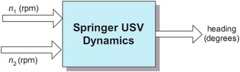
Figure 1. Block diagram representation of a two-input USV.
The vehicle has a differential steering mechanism and thus requires two inputs to adjust its course. This can be simply modelled as a two input, single output system in the form depicted in Figure 1, where n 1 and n 2 are the two propeller speeds in revolutions per minute (rpm). Clearly, straight-line manoeuvres require both the thrusters running at the same speed, the differential thrust being zero in this case. In order to linearize the model at an operating point, it is assumed that the vehicle is running at a constant speed. To clarify this further, let n c and n d represent the common mode and differential mode thruster velocities defined as:
 $$\left. \matrix{n_c = \displaystyle{{n_1 + n_2} \over {\rm 2}} \cr n_d = \displaystyle{{n_1 - n_2} \over {\rm 2}}} \right\}$$
To maintain the velocity of the vessel, n c must remain constant at all times. During trials, a forward speed of three knots was maintained, which corresponds to a constant value of n c = 900 rpm.
The differential mode input, however, oscillates about zero depending on the direction of the manoeuvre. For data acquisition, several inputs were superimposed with a pseudo-random binary sequence to excite the system's dynamics and were applied to the thrusters. The corresponding heading response was collated, and SI was then applied to the acquired data from which a dynamic model for the steering of the vehicle was obtained in the following form (Naeem et al., Reference Naeem, Xu, Sutton and Tiano2008):
 $${\bi x}{\rm (}k + {\rm 1)} = {\bf A}\,{\bi x}{\rm (}k{\rm )} + {\bf B}\,u{\rm (}k{\rm )}$$
 $$y{\rm (}k{\rm )} = {\bf C}\,{\bi x}{\rm (}k{\rm )}$$
where
 $${\bf A}{\rm} = \left[ {\matrix{ {1.002} & 0 \cr 0 & {0.9945} \cr}} \right],{\bf B} = \left[ {\matrix{ {6.354} \cr { - 4.699} \cr}} \right] \times 10^{ - 6}, {\bf C}{\rm} = \left[ {\matrix{ {{\rm 34}{\rm. 13}} & {{\rm 15}{\rm. 11}} \cr}} \right]$$
with a sampling time of 1 s, where u(k) represents the differential thrust input in rpm and y(k) the heading angle in radians. Cross-correlation and autocorrelation tests were carried out to validate the model (Naeem et al., Reference Naeem, Xu, Sutton and Tiano2008).
2.2 Compass Dynamics
A dynamic model for the TCM2 compass has already been derived through SI techniques (Xu, Reference Xu2007) and is given by the following hybrid stochastic-deterministic state-space model
 $${\bi x}{\rm (}k + {\rm 1)} = {\bf A}\,{\bi x}{\rm (}k{\rm )} + {\bf B}\,u{\rm (}k{\rm )} + {\bi \omega} {\rm (}k{\rm )}$$
 $$y{\rm (}k{\rm )} = {\bf C}\,{\bi x}{\rm (}k{\rm )} + \upsilon {\rm (}k{\rm )}$$
where
 $$\eqalign{& {\bf A}{\rm} = \left[ {\matrix{ {0.2796} & {0.6971} \cr 1 & 0 \cr}} \right],{\bf B} = \left[ {\matrix{ {0.4364} \cr 0 \cr}} \right],{\bf C}{\rm} = K\left[ {\matrix{ {\rm 1} & {\rm 0} \cr}} \right] \cr & cov{\rm (}{\bi \omega} {\rm )} = diag{\rm \{ 1,1\},} \quad \sqrt {var(\upsilon )} = {\rm 2}{\rm ^\circ}} $$
with a sampling period of 0·025 s. The input to the model is the actual heading of the vessel, in degrees, and the output is the compass measurement, also in degrees, whereby it can be assumed that the constant K is such that the steady state gain of the model is unity (resulting in K = 0·05339). Correlation tests were carried out to validate the model.
3. THE NAVIGATION SYSTEM
The navigation system of the vehicle is concerned with estimating the actual heading angle of the vessel at each sampling time. The approach used here is based on Kalman filtering: firstly, the standard KF is described in this section, and secondly, a novel approach based on the wIKF is presented.
3.1 Kalman Filter
For linear systems governed by stochastic-deterministic state-space equations such as Equations (5) and (6), it is well established that the KF provides statistically optimal estimates of the state vector from measured data. The KF equations implemented in this study can be found in Motwani et al. (Reference Motwani, Sharma, Sutton and Culverhouse2013b).
Despite its widespread use, the optimal nature of the KF relies upon an accurate description of the dynamic model and system and measurement noise covariances. An example of the effects of erroneous modelling on the heading estimate for the Springer was shown in Motwani et al. (Reference Motwani, Sharma, Sutton and Culverhouse2013b), in which accurate KF estimates were only obtained if the model description was accurate as well. This causes a significant inconvenience, as this is seldom the case in practice, especially for processes susceptible to being affected by numerous external factors.
In order to reproduce such a non-idealistic scenario, assume that all the coefficients of Equation (7) have been underestimated by 0·5%, and that the actual compass dynamics are given instead by:
 $$\eqalign{& {\bf A} = 1.005 \times \left[ {\matrix{ {0.2796} & {0.6971} \cr 1 & 0 \cr}} \right], {\bf B} = 1.005 \times \left[ {\matrix{ {0.4364} \cr 0 \cr}} \right],{\bf C} = K \left[ {\matrix{ 1 & 0 \cr}} \right], \cr & \quad\quad\quad\quad\quad\quad\quad\quad \quad \quad K = 1.0050 \times 0.05339 \cr & \quad \quad\quad\quad\quad \quad \quad cov({\bi \omega} ) = diag\{ 1,1\}, \quad \sqrt {var(\upsilon )} = 2^{\circ}} $$
This change of behaviour could be the result, for instance, of an unaccounted for weak external magnetic field that is biasing the compass readings, or it could be that the model obtained in Equation (7) may have resulted from fitting data gathered under non-ideal conditions.
In either case, it should be noted that even though the model assumed by the KF (given by Equation (7)) does not reflect the true compass dynamics, the compass measurements simulated in this study are generated according to the actual compass dynamics given by Equation (8).
3.2 Weighted Interval Kalman Filter
The application of interval Kalman filtering to the navigation of USVs was discussed in detail in Motwani et al. (Reference Motwani, Sharma, Sutton and Culverhouse2013b), which also described the principles of the IKF. However, for completeness, a brief summary of the concepts behind the IKF are given here.
When system dynamics are not known precisely, but known to lie within finite bounds, a version of the KF known as the IKF may be adopted, capable of providing rigorous bounds to the optimal state estimate. The algorithm was first proposed by Chen et al. (Reference Chen, Wang and Shieh1997), and can be summarised as follows.
Let A, B and C contain elements which are uncertain within some definite bounds. The system can then be described by:
 $${\bi x}{\rm (}k + {\rm 1)} = {\bf A}^{\bf I} {\bi x}{\rm (}k{\rm )} + {\bf B}^{\bf I} u{\rm (}k{\rm )} + {\bi \omega} {\rm (}k{\rm )}$$
 $${\bi y}{\rm (}k{\rm )} = {\bf C}^{\bf I} {\bi x}{\rm (}k{\rm )} + {\bi \upsilon} {\rm (}k{\rm )}$$
where  ${\bf M}^{\bf I} = {\bf M} \pm {\rm \Delta} {\bf M} = {\rm [}{\bf M} - \left\vert {{\rm \Delta} {\bf M}} \right\vert{\rm,} \;\;{\bf M} + \left\vert {{\rm \Delta} {\bf M}} \right\vert{\rm ]}$ for ${\bf M} \in {\rm \{} {\bf A}{\rm,} {\bf B}{\rm,} {\bf C}{\rm \}} $, and ω(k) and υ(k) are white noise sequences with zero-mean Gaussian distributions with known covariances cov(ω) = Q, cov(υ) = R, and E[ω(l) υT(k)] = 0 $\forall $l,k, E[x(0) ω T(k)] = 0, E[x(0) υ T(k)] = 0 $\forall $k.
The IKF algorithm is given by the recursive Equations (11) to (15), which mimic those of the ordinary KF but are described in terms of intervals. Given an initial estimate  $\hat{\bi x}^{\bi I} {\rm (}0{\rm )}$ and its uncertainty, characterised by ${\rm P}^{\rm I} {\rm (}0{\rm )} \equiv {\rm } v{\rm ar}[\hat{\bi x}^{\bi I} {\rm (}0{\rm )]}$, together with the input to the system and the output measurement at each time-step, the resulting state estimate is an interval vector $\hat{\bi x}^{\bi I} {\rm (}k{\rm )}$ at each time-step k, providing an upper and lower boundary to the estimate, as illustrated in Figure 2.
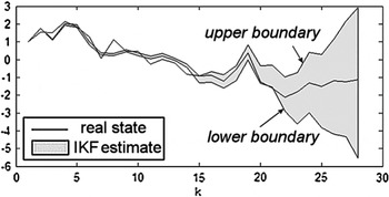
Figure 2. IKF estimate depicting its upper and lower boundaries.
Prediction:
 $$\hat{\bi x}^{{\bi I -}} {\rm (}k + 1{\rm )} = {\rm} {\bf A}^{\bf I} \hat{\bi x}^{{\bi I} +} {\rm (}k{\rm )} + {\bf B}^{\bf I} u{\rm (}k{\rm )}$$
 $${\rm P}^{{\rm I -}} {\rm (}k + 1{\rm )} = {\rm} {\bf A}^{\bf I} {\rm P}^{{\rm I} +} {\rm (}k{\rm )} {\bf A}^{{\bf I}^{\bf T}} + {\rm Q}$$
Kalman Gain:
 $${\rm K}^{\rm I} {\rm (}k{\rm )} = {\rm} {\rm P}^{{\rm I -}} {\rm (}k{\rm )} {\bf C}^{{\bf I}^{\bf T}} \left\{ {\left. {{\bf C}^{\bf I} {\rm P}^{{\rm I -}} {\rm (}k{\rm )} {\bf C}^{{\bf I}^{\bf T}} + {\rm R}{\rm (}k{\rm )}} \right\}} \right.^{ - 1} $$
Correction:
 $$\hat{\bi x}^{{\bi I} +} {\rm (}k{\rm )} = {\rm} \hat{\bi x}^{{\bi I} -} {\rm (}k{\rm )} + {\rm} {\rm K}^{\rm I} {\rm (}k{\rm )} [{\bi z}{\rm (}k) - {\bf C}^{\bf I} \hat{\bi x}^{{\bi I -}} {\rm (}k)]{\rm} $$
 $${\bf P}^{{\bf I} + {\bf}} {\rm (}k{\rm )} = {\rm [}{\rm} {\bf I}{\rm -} {\bf K}^{\bf I} {\rm (}k{\rm )}{\bf C}^{\bf I} {\rm ]}{\bf P}^{{\bf I} - {\bf}} {\rm (}k{\rm )} $$
in which z(k) is the measurement at time k, that is to say, a particular realisation of y(k).
In order to increase the robustness of the KF, an IKF that uses an interval model is employed. This interval model is such that it contains a range of point-valued models which are centred around the nominal model given by Equation (7). Specifically, assume that the coefficients in Equation (7) are known to be accurate to within 1% of the nominal values. Then the following interval model can be adopted:
 $${\bi x}{\rm (}k + {\rm 1)} = {\bf A}^{\bf I} {\bi x}{\rm (}k{\rm )} + {\bf B}^{\bf I} u{\rm (}k{\rm )} + {\bi \omega} {\rm (}k{\rm )}$$
 $${\rm y}{\rm (}k{\rm )} = {\bf C}^{\bf I} {\bi x}{\rm (}k{\rm )} + {\rm \upsilon} {\rm (}k{\rm )}$$
with
 $$\eqalign{& {\bf A}^{\bf I} = \left[ {\matrix{ {[0.9 \times 0.2796,\,\,1.1 \times 0.2796]} & {[0.9 \times 0.6971,\,\,1.1 \times 0.6971]} \cr {[0.9,\,\,1.1]} & 0 \cr}} \right], \cr & {\bf B}^{\bf I} = \left[ {\matrix{ {[0.9 \times 0.4364,\,\,1.1 \times 0.4364]} \cr 0 \cr}} \right],{\bf C}^{\bf I} = K\left[ {\matrix{ {[0.9,\,\,1.1]} & {\rm 0} \cr}} \right], \cr & K = {\rm} 0.05339;\quad cov{\rm (}{\bi \omega} {\rm )} = diag{\rm \{ 1,1\},} \quad \sqrt {var(\upsilon )} = {\rm 2}{\rm ^\circ}} $$
Note that this interval model includes the true compass dynamics given by Equation (8). Also, as noted previously, the measurements generated via simulation are point-valued measurements from the actual compass dynamics (Equation (8)) rather than generated from Equation (17).
Implementation of the IKF algorithm requires the use of interval arithmetic, which tends to yield overly conservative bounds. As discussed in Motwani et al. (Reference Motwani, Sharma, Sutton and Culverhouse2013b), the calculated bounds tend to diverge due to the so-called “dependency effect” of interval arithmetic. In order to minimise this effect, the IKF expressions involving interval variables may be reformulated in several ways to take advantage of different factorisations, and the intersection of the resulting values computed using each one of these will provide the smallest interval that contains the true result. This constitutes a simple and effective procedure to sharpen interval computations, and is the method adopted here in obtaining the IKF interval estimates.
Once the IKF bounds are obtained, nonetheless, in practice a single point-valued estimate is desired. Chui and Chen (Reference Chui and Chen2008) proposed obtaining a weighted average of the boundaries, and this method is adopted here. The weighted average, or wIKF estimate, is given by
 $$\hat h_{wIKF} (k) = \hat h_{wIKF}^{\inf} (k) + w(k) [\hat h_{wIKF}^{\sup} (k) - \hat h_{wIKF}^{\inf} (k)]$$
where  $\hat h$ denotes heading estimate, and the superscripts sup and inf refer to the upper and lower bounds of the IKF estimate.
In this study, as well as the wIKF, an ideal KF is simulated in parallel. It is ideal in the sense that it adopts the true model of the compass (Equations (5) to (7)). The wIKF weight is then calculated at each time step as that which is necessary for the weighted average of the IKF bounds to coincide with the ideal KF estimate. In other words,
 $$w(k) = {\rm} \displaystyle{{\hat h^{ideal} (k) - \hat h_{wIKF}^{\inf} (k)} \over {\hat h_{wIKF}^{\sup} (k) - \hat h_{wIKF}^{\inf} (k)}}$$
Although an ideal KF is simulated in order to compute this weight, it is possible to obtain a good approximation of the same without the need of an ideal KF, as will be noted in the ensuing discussion.
4. THE GUIDANCE SYSTEM
Different guidance strategies used in marine environments to guide the vehicles are further illustrated in Annamalai (Reference Annamalai2012). The most popular guidance strategy is waypoint LOS strategy and this is utilised here. It is briefly illustrated as follows.
Based on the current estimated position of the USV and the coordinates of the next waypoint to be reached, the desired or reference heading angle based on LOS is calculated as follows:
 $$r(k) = arctan \left( {\displaystyle{{y_d (k) - y(k)} \over {x_d (k) - x(k)}}} \right)$$
where (x, y) is the current location of the vessel and (x d, yd) the target coordinates. In practice, because the inverse of the tangent is restricted to (−90°, 90°), the four quadrant inverse tangent, arctan2[y d(k)-y(k), x d(k)-x(k)], which takes into account the signs of both arguments, is used instead. Also, as the reference (or desired) heading angle changes, care is taken to ensure that the vehicle is directed to turn toward it in the direction that requires the lesser total change in its own heading, since two possibilities always exist.
The guidance system keeps track of the mission status, which includes a log of the waypoints reached or missed and the current target waypoint, as well as the total distance travelled, deviation from the ideal trajectory, and controller energy consumed. These are updated every sampling instant based on the current position of the USV. All of these concepts are described next.
To decide whether a waypoint has been reached or not, the guidance system considers a Circle Of Acceptance (COA) around each waypoint (Figure 3). A COA is needed since the marine environment is continuously moving with some degree of randomness, making it unfeasible in practice to target a single point precisely. Healey and Lienard (Reference Healey and Lienard1993) suggested that the radius of the COA should be at least twice the length of the vehicle. However, their concern was to do with underwater vehicles. Since surface vessels benefit from GPS localisation, a radius equal to the length of the vessel is deemed sufficient in the present investigation. For Springer the length is approximately 4 m, thus this is the radius assigned to the COA.

Figure 3. Deviation at time k.
At each sampling instant, the guidance system calculates the distance left to the next waypoint according to
 $$\rho = \sqrt {[x_d (k) - x(k)]^2 + [y_d (k) - y(k)]^2} \le \rho _0 $$ $\rho _0 $ being the radius of the COA. When this condition is met, it is regarded that the waypoint is reached, and the guidance system directs the vessel to the next waypoint.
However, the vessel might pass by the vicinity of a waypoint without entering the COA. This condition is determined by checking the derivative  $d\rho /dt$, which when it switches from negative to positive, indicates that the vessel has missed the waypoint. In this case, the guidance system also directs the vessel toward the next waypoint.
The vessel normally follows a path different from the ideal one. Several performance indices are used to assess the trajectories followed, which the guidance system computes at each time step and keeps track of. The deviation from the ideal trajectory can be measured as
 $$rd(k) = \sqrt {\;\overline {PB} ^2 + \;\overline {P{\kern 1pt} {\kern 1pt} ^{\!\prime}B} ^2 - \;2\,\,\overline {PB} \, \cdot \overline {P{\kern 1pt} {\kern 1pt} ^{\!\prime}B} \;\cos (\alpha )} $$
where  $\overline {PB} $ is the distance, at time k, to the next waypoint from the position of the vehicle were it on the ideal path, and $\overline {P{\kern 1pt} {\kern 1pt} ^{\prime}B} $ the distance to the next waypoint from its actual position at time k, α being the angle between the two vectors, as shown in Figure 3.
Finally, the average controller energy  $\overline {CE_u} $ is defined as
 $$\overline {CE_u} = \displaystyle{{\sum\limits_{k\, = \,1}^N {\,[{{u_c (k)} / {60]^2}}}} \over N}$$
where N is the total number of time steps and u c the controller effort at time k in rpm.
5. THE CONTROL SYSTEM
The concepts and techniques of MPC have been developed over the past three decades (Annamalai, Reference Annamalai2012), and various authors such as Maciejowski (Reference Maciejowski2002), Rawlings and Mayne (Reference Rawlings and Mayne2009), Wang (Reference Wang2009) and Allgower et al. (Reference Allgower, Glielmo, Guardiola and Kolmanovsky2010) suggest that MPC is widely used in the process and petrochemical industries. In addition, the marine control system design fraternity has also embraced this approach since it offers the advantage of being capable of enforcing various types of constraints on the plant process as exemplified by Naeem et al. (Reference Naeem, Sutton, Chudley, Dalgleish and Tetlow2005), Perez (Reference Perez2005), Oh and Sun (Reference Oh and Sun2005), Liu et al., (Reference Liu, Allen and Yi2011) and Li and Sun (Reference Li and Sun2012).
In general, the plant output is predicted by using a model of the plant to be controlled. Any model that describes the relationship between the input and the output of the plant can be used. Further if the plant is subject to disturbances, a disturbance or noise model can be added to the plant model. In order to define how well the predicted process output tracks the reference trajectory, a criterion function is used. Typically the criterion or cost function is of the following form,
 $$J = \;\sum\limits_{i = 1}^{H_p} {e(k + i)^T Q\,e(k + i) +} \sum\limits_{i = 1}^{H_c} {\Delta u(k + i)^T R\,\Delta u(k + i)} $$
subject to,
 $$\Delta u^l \le \Delta u(k + i) \le \Delta u^u $$
where  $\,e(k) = \hat y\,(k) - r(k)$ is the prediction error, or difference between the predicted process output $\hat y$ and the reference trajectory r. The superscripts l and u represent the lower and the upper bounds respectively. Q is the weight on the prediction error, and R the weight on the change in the input Δu. H p is the prediction horizon or output horizon, and H c the control horizon. More details can be found in Naeem et al. (Reference Naeem, Sutton, Chudley, Dalgleish and Tetlow2005). For completeness, the general structure of an MPC is shown in Figure 4(a).

Figure 4. MPC (a) General structure; (b) General strategy.
The optimal controller output sequence u opt over the prediction horizon is obtained by minimisation of J with respect to u. As a result the future tracking error is minimised.
The MPC algorithm consists of the following three steps.
• Step 1. Use a model explicitly to predict the process output along a future time horizon (Prediction Horizon).
• Step 2. Calculate a control sequence along a future time horizon (Control Horizon, H c), to optimise a performance index.
• Step 3. Employ a receding horizon strategy so that at each instant the horizon is moved towards the future, which involves the application of the first control signal of the sequence calculated at each step. The strategy is illustrated in Figure 4(b).
In Figure 4(b), the predicted output and the corresponding optimum input over a horizon H p are shown, where u(k) is the optimum input,  $\hat{y}(k)$(k) is the predicted output, and y(k) the process output.
The controller is not fixed and is designed at every sampling instant based on actual sensor measurements so disturbances can easily be dealt with as compared to fixed gain controllers.
For the integrated NGC system in Springer, an MPC was chosen as autopilot since previous studies (Annamalai and Motwani, Reference Annamalai and Motwani2013) have shown that it provides better performance than more standard approaches such as linear quadratic Gaussian-based controllers. The plant model used by the MPC algorithm is the model of the vehicle described in Section 2.1 (Equations (2) to (4)), the input u(k) being the differential mode thruster velocity n d (k), and the output y(k) corresponding to the heading of the vehicle, which in the integrated NGC system is provided by the KF/wIKF estimate rather than assumed to be directly available, as this would not be the case in practice.
The MPC controller also incorporates the actuator limitations of the vessel as optimisation constraints. These are given by
 $$\left\vert {n_d} \right\vert \le 300\;rpm\; \; {\rm and} \; \left\vert {\Delta n_d} \right\vert \le 20\,rpm$$
that is, a limitation both on the maximum absolute value and on the change of the rpm of the motors from one sampling instant to the next.
The parameters of the MPC algorithm used are H p = 10 and H c = 2, as these values were found to be optimal, and the weights Q = 1 and R = 0·1 were chosen for the cost function. Further rationale for the choice of these parameters can be found in Annamalai (Reference Annamalai2014).
6. RESULTS AND DISCUSSION
The block diagram shown in Figure 5 illustrates the integration of the three subsystems.
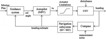
Figure 5. NGC system block diagram.
The mission plan consists of the set of predefined waypoints through which it is desired for the vessel to traverse. The particular mission plan used herein consists of seven waypoints forming a closed circuit (Figures 7(a) and 9(a)). Based on the mission plan and current location of the vehicle (assumed to be known), the guidance system (described in detail in Section 4) keeps track of previous and next-waypoints, distance travelled and remaining, etc. It also generates the desired (or reference) heading angle as the angle of the straight line connecting the vessel's current estimated position and the next waypoint. (Angles are with respect to a reference direction, in this case Due East, given by the x-axis in Figures 7(a) and 9(a)). In turn, based on the desired heading angle and the current estimated heading of the vehicle, the autopilot, or controller, generates the most adequate control signal, or differential thrust of the motors (recall that steering is controlled via the differential mode thruster velocity, n d). The autopilot here is concerned only with heading control, since, as was previously stated, the common mode thruster velocity n c is maintained constant throughout.
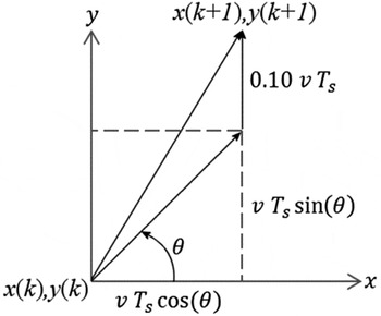
Figure 6. Velocity triangle.
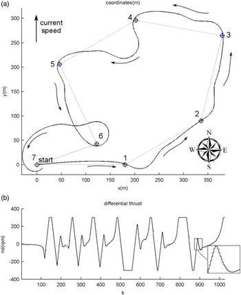
Figure 7. Simulations corresponding to the NGC system with KF based on incorrect TCM2 model; (a) trajectory, (b) MPC output.
The position of the vessel at each time step is calculated from the previous position using dead reckoning, given that the forward speed of the vessel (relative to the water surface) is constant and known. Added to this, a constant disturbance consisting of an added velocity of 10% of the forward speed of the vehicle, acting in a northerly direction, was added to consider the effect of surface currents (Figure 6). If x(k) and y(k) represent the position of the vessel at time k, then the position at the next sample time is calculated as follows:
 $$x{\rm (}k + 1{\rm )} = {\rm} x{\rm (}k{\rm )} + {\rm} v\;T_s \,{\rm cos(}\theta {\rm )}$$
 $$y{\rm (}k + 1{\rm )} = {\rm} y{\rm (}k{\rm )} + {\rm} v\;T_s \,\sin {\rm (}\theta {\rm )} + {\rm 0}{\rm. 10}\,v\;T_s $$
where v is the constant forward speed of the vessel (3 knots), T s the sampling interval of 1 s, θ the actual heading angle of the vessel at time k, and  ${\rm 0}{\rm. 10}\,v\;T_s $ the effect of the surface current disturbance which is added to the y component of the vehicle's position.
The actual heading of the vessel is generated according to Equations (2) to (4), with the added random input ω(k) in the state equation (Equation (2)), rendered as a random Gaussian white noise sequence with zero mean and covariance diag{1,1}×10−14, and which models the random effects of surface waves. It is shown in Figure 5 as a disturbance that affects the heading of the vessel.
The waypoint-tracking mission was simulated using two different approaches that differ in the navigation system used. In both cases, LOS and MPC, as described in the previous sections, were used for guidance and control of the vehicle, as these methods constitute realistic strategies that have been proven to be effective in this area (Annamalai and Motwani Reference Annamalai and Motwani2013, Naeem et al., Reference Naeem, Sutton and Chudley2006), and are thus maintained for this study.
For the navigation system, firstly, a KF based on the incorrect nominal model of the TCM2 compass dynamics (Equation (7)) was used to estimate the heading of the USV. Figure 7(a) shows the trajectory followed by the vehicle, while Figure 7(b) shows the controller output. Note that the generated control signal is within the prescribed actuator limits.
Figure 8 shows the reference heading generated by the guidance system, as well as the true heading of the vehicle and the KF estimate of the same. It can be observed from the figure that the estimated heading does not converge to the mean value of the actual heading, since the incorrect compass model used in the KF is biased. This inaccuracy in the estimated heading in turn affects the guidance and control systems, as can be observed from the somewhat winding trajectory followed by the vehicle in this case (Figure 7(a)). In particular, the KF tends to overestimate the heading of the vehicle, increasingly so during the latter part of the course (Figure 8). The effect of this is that the vehicle tends to miss waypoints, bypassing them to its left, because its actual heading falls short of what it should be (the KF estimate) to target the waypoint exactly. This is apparent in Figure 7(a) in which the vehicle misses the last four waypoints.
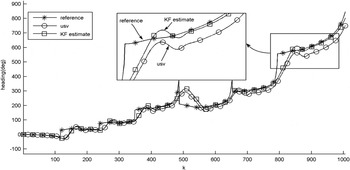
Figure 8. Comparison of reference heading, actual vehicle heading, and estimated heading, using KF based on incorrect TCM2 model. (a) Way point tracking using wIKF. (b) Controller output n d.
In the second instance, a wIKF was used to estimate the heading of the USV, as described in Section 3.2. Figures 9(a) and 9(b) show the trajectory followed by the vehicle, and the MPC control output, respectively. Figure 10 shows the reference heading and compares the actual heading of the vehicle with the estimated one. It can be observed that the estimated heading matches the true heading much more closely than in the previous case, and this translates into a much smoother and more efficiently generated trajectory, as evidenced in Figure 9(a).

Figure 9. Simulations corresponding to the NGC system with wIKF heading estimate; (a) trajectory, (b) MPC output.
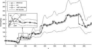
Figure 10: Comparison of reference heading, actual vehicle heading, and estimated heading from wIKF.
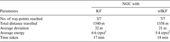
From the two simulations described, global performance parameters were obtained and are summarised in Table 1. The number of waypoints reached reflects only those for which the vehicle entered the COA. In the case of navigation using the KF, four out of the seven waypoints were not reached (namely waypoints 4, 5, 6, and 7), although the vehicle was directed to the next target when it was detected to have passed one without entering the COA. In the case of the system using the wIKF navigation estimate, all waypoints were reached. The wIKF NGC system also achieved better performance in terms of distance travelled (13% reduction), deviation from the ideal trajectory (34% less), energy used (18% lower) and time taken (18% less).
Table 1. Comparison of performance parameters.
The preceding results highlight the importance of accurate navigation for the USV mission as a whole. The improved heading estimate accuracy can be evidenced by comparing Figures 8 and 10. A comparison of the navigational accuracy is explicitly shown in Figure 11, which shows the errors (difference between true and estimated heading) of the two navigation systems. In fact, by definition of the weights used, generated according to Equation (19), the wIKF estimates are equal to the KF estimates that would have been obtained had the true model of the compass been used.
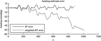
Figure 11. Comparison of wIKF and traditional KF estimation errors.
Although in order to calculate the ideal weightings for the wIKF, estimates from an ideal KF were used, in practice the true dynamics of the system will not generally be known precisely. However, studies have shown that it is possible to infer these ideal weights without knowledge of the true system dynamics, and hence, without relying on the estimates of an ideal KF. Motwani et al. (Reference Motwani, Sharma, Sutton and Culverhouse2013a) devised a method based on using data generated in a simulation study such as this one to train a neural network to predict the optimum weights. The idea is basically the following: one can construct a simulation mission and adopt some model to simulate the readings of the compass, which will thus represent the “true” compass dynamics for that simulation. The chosen compass dynamics must be some model contained in the interval model of the compass (which is what is only known in reality). One can then simulate an IKF, an ideal KF (that is, based on the model chosen to simulate the compass), and some nominal KF (whose model differs from that of the one used to simulate the compass, although still contained in the interval model). Based on these simulations, the neural network is then trained to correlate the innovations sequence of the nominal KF (which is an indicator of its performance) with the desired wIKF weight (calculated by Equation (20)). The trained neural network is then capable of estimating this desired weight for new missions based on the innovations of any nominal KF contained in the interval model, regardless of what the actual dynamics of the compass are (as long as they are contained in the interval model). Hence, the method itself does not rely on knowledge of the true system dynamics, but only upon being able to describe it via an interval model such as the one given by Equation (18). Thus, the arguments presented in this paper are justified even though, for the sake of conciseness and clarity, the weights of the wIKF were generated by Equation (20).
It should be emphasised that in practice, computing the wIKF estimates requires running both a KF and an IKF in parallel, as well as a neural network for predicting the optimal weight. The IKF uses exactly the same formulation as that of a regular KF, but operates on interval values instead. In practice, this means that an interval arithmetic needs to be implemented on a computer. There are many programming languages that incorporate interval data types nowadays; in particular, the simulations shown in this paper were computed using the open-source extension of MATLAB for interval arithmetic, INTerval LABoratory (INTLAB), developed by Rump (Reference Rump1999). Using INTLAB, the computational overhead of dense matrix multiplication for interval valued elements translates into an estimated timing factor of between five and ten compared to pure floating-point matrix multiplication. Regarding the computation of the weight, it should be noted that the training of the neural network is done on a training data set, offline. The actual use of the trained network for predicting the weight typically requires two matrix multiplications at each time-step (in the case of a layered perceptron model with a single hidden layer), that is, O(N3) floating point operations for each one, N being the order of the matrix.
7. CONCLUDING REMARKS
To summarise, the waypoint tracking capability of an innovative integrated NGC system for an USV is explored in this paper. The Springer used as the test platform is described briefly and system identification is used to capture the yaw dynamics of the USV and to model a TCM2 electronic compass used on board the vehicle. These models are respectively used by the predictive autopilot and KF-based navigation systems. Navigation based on a KF using a biased compass model and another based on a wIKF are simulated to complete the waypoint tracking mission. In both cases, a waypoint LOS guidance system is utilised to generate the reference trajectory, and an MPC autopilot as the control system to keep the vehicle on course. The performances of the two integrated systems are compared.
The key aspect of this paper is to show how the novel wIKF can be used effectively in conjunction with the aforementioned guidance and control systems, and that it provides a navigation system that is robust to (a finite amount of) uncertainty in the model it relies upon. This in turn has a marked effect, improving the accuracy and efficiency of the integrated NGC system as a whole for the completion of the mission, leading to better overall results in terms of total distance travelled, deviation, energy and time consumed, and not least, the actual number of waypoints successfully tracked by the vehicle. This technique constitutes a novel approach to address the increasing demand for autonomous capabilities in cost-effective USV platforms such as Springer that relies on software-based techniques to enhance the effectiveness and reliability of its relatively low-budget sensors and restricted modelling facilities.


