1. INTRODUCTION
The assessment of clear space around the ship is of major importance for safe navigation. A recent research conducted by the Nautical Institute (NI) indicated that 60 per cent of collision and grounding cases are caused by direct human error (Gale and Patraiko, Reference Gale and Patraiko2007) and the two major human related causes are “insufficient assessment of the situation” (24%) and “poor look out” (23%). To assess the situation, navigators often adopt a set of safety criteria such as the Distance at Closest Point of Approach (DCPA) and Time to Closest Point of Approach (TCPA) to determine if actions need to be taken. Another popular safety criterion, which was first proposed by Fujii and Tanaka (Reference Fujii and Tanaka1971) is the use of ship domain – a physical spacing around the ship to ensure sufficient separation between ships. Ship domain has been adopted in collision-risk assessments (Fujii and Tanaka, Reference Fujii and Tanaka1971; Goodwin, Reference Goodwin1975; Pietrzykowski, Reference Pietrzykowski2008; Pietrzykowski and Uriasz, Reference Pietrzykowski and Uriasz2009), collision-avoidance pre-emption (Dove et al., Reference Dove, Burns and Stockel1986; Zhao et al., Reference Zhao, Tan, Price and Wilson1994), traffic simulation (Davis et al., Reference Davis, Dove and Stockel1980; Coldwell, Reference Coldwell1983; Hansen et al., Reference Hansen, Jensen, Lehn-Schiøler, Melchild, Rasmussen and Ennemark2013), as well as navigational path planning (Smierzchalski and Michalewicz, Reference Smierzchalski and Michalewicz2000; Szlapczynski, Reference Szlapczynski2011).
A number of shapes have been proposed to represent the ship domain. Goodwin (Reference Goodwin1975) and Davis et al. (Reference Davis, Dove and Stockel1980) proposed circular domains while Fujii (Reference Fujii and Tanaka1971), Coldwell (Reference Coldwell1983) and Kijima (Reference Kijima and Furukawa2003) preferred elliptical domains and others, for example, Smierzchalski (Reference Smierzchalski2000) and Pietrzykowski (Pietrzykowski, Reference Pietrzykowski2008; Pietrzykowski and Uriasz, Reference Pietrzykowski and Uriasz2009) used polygonal domains. While regularly-shaped domains may be simple to describe and apply, they often do not adequately represent all the navigational encounters well. On the other hand, domains using complex shapes are difficult to determine, particularly if the calibration process is not rigorous.
To determine ship domains, statistical methods have been initially used, although most ship domains have not been well calibrated. The ship domains based on statistical approaches usually rely on data of ship movement trajectories (Fujii and Tanaka, Reference Fujii and Tanaka1971; Goodwin, Reference Goodwin1975; Coldwell, Reference Coldwell1983). However, while the trajectory data are suitable for studies of traffic capacity and channel navigation safety (Zhao et al., Reference Zhao, Wu and Wang1993), their use in ship domain analysis were not well established. In addition, three shortcomings of statistical methods for obtaining ship domains have been identified by Pietrzykowski and Uriasz (Reference Pietrzykowski and Uriasz2009): 1) necessity for sufficient amount of data, 2) difficulties in separating the factors affecting the domain shape and size and 3) an unclear description of the perceived clear area around the ship. Therefore the statistical methods for developing ship domains still have room to improve, although Hansen et al. (Reference Hansen, Jensen, Lehn-Schiøler, Melchild, Rasmussen and Ennemark2013) recently attempted to overcome these shortcomings by using a large number of observations from the Automatic Identification System (AIS).
In general, navigational waters can be divided into three categories: 1) open sea waterways, 2) confined waterways and 3) narrow fairways and channels. Most of the existing ship domains are developed for open waters (Goodwin, Reference Goodwin1975), while very few are for narrow fairways and confined waters (Fujii and Tanaka, Reference Fujii and Tanaka1971; Pietrzykowski, Reference Pietrzykowski2008). The traffic densities in the three categories of waterways are significantly different. Empirically, Goodwin (Reference Goodwin1975) found that the size of ship domain is dependent on ship density and the operating environment. While there are more degrees of freedom in open oceans than in congested strait waters, it is debatable that a substantially larger ship domain is necessary for open waters or that the resulting size is limited by the lack of critical close encounters in open waters. On the other hand, in narrow fairways, the ship domain may be constrained by the fairway geometry or ship turning ability rather than just traffic influence and navigational behaviour (Pietrzykowski, Reference Pietrzykowski2008). Consequently, the trajectory data may be rather biased by fairway geometry to enable a fair representation of the ship domain. A study on ship domain using data in confined waters is most promising but there are only a few studies available, e.g., Hansen et al. (Reference Hansen, Jensen, Lehn-Schiøler, Melchild, Rasmussen and Ennemark2013).
Navigation within confined waters is influenced not just by traffic density in the area but also the presence of general as well as locally-imposed traffic rules. One of the principal rules in navigation is the International Regulations for Preventing Collisions at Sea 1972 (COLREGS, 1972), which stipulate give-way and stand-on behaviours according to specific ship encounters. For most ship domain models, the definitions of ship encounter are crude. For instance, they are usually grouped into three broad encounters, i.e., overtaking (or being overtaken), head-on and crossing, according to the relative heading and bearing. This results in an undesirable abrupt change in safety criterion at the interface between two encounter types due to a change in relative heading and bearing.
To overcome the above limitations, a rigorous approach to modelling ship domains in confined waters is proposed. This paper has developed a free-form ship domain for risk assessment in confined waters. The methodology for developing and evaluating the model is described in Section 2. The calibrated model of ship domain is presented in Section 3, which is followed by a discussion of the proposed model in Section 4. Section 5 summarises the key findings of this research and highlights the potential areas for future work.
2. METHODOLOGY
2.1. Formulation of Ship Domain
To take into account attributes of both ships in an encounter, the safe spacing that the ships will keep from each other is modelled to comprise two components; one belonging to the Own Ship (OS) and the other Target Ship (TS). Further, since the safe spacing is also influenced by the heading of the two ships, we then formulate the concept of two individual ship domains around the ship, the size of which is dependent on the Length Overall (LOA) and the current speed. The safe distance which both ships will keep from each other is considered as the sum of the length of each of the domains (i.e., SDOS and SDTS for OS and TS respectively shown in Figure 1) in the direction of the line of sight between the ships. Conceptually, it is as though ships will navigate to ensure the two individual domains will not encroach into each other. We consider the two individual ship domains to assume a unified domain model determined by its ship attributes and calibrated using observed navigational data.

Figure 1. Definition of safe spacing.
The proposed perspective should effectively represent the safe navigational water between approaching ships, and reflect the navigational features of both ships and their interactive navigational behaviour. Instead of adopting a simplified and restricted elliptical domain around each ship, this study assumes an asymmetrical polygonal shape with small discretized intervals, thus offering it a higher degree of freedom. In addition to relaxing the limitation on the shape, the size of the ship domain will be dynamically enlarged with increasing ship speed based on a consistent basis of the domain. Furthermore, the required safe distance between ships governed by the edge of the ship domain will also change with changing relative bearing and heading throughout the encounter. Based on this concept, the domain model will include three components: the representation of domain shape, the representation of the basic domain size for the stationary ship and finally the effect of the ship speed function.
The individual domain is defined in the shape of an asymmetrical polygon with n number of vertices and the boundary of the domain is formed by joining the n vertices sequentially. The size of the polygon is measured by the radial distance R from the ship centre to the different vertices of the polygon, defined by a polar angle θ i clockwise from the ship heading and it is governed by a function of ship LOA (L) and speed (v):
 $$R_{\theta _i} = \alpha _{\theta _i} \cdot L \cdot g_{\theta _i} \left( v \right)$$
where i (i = 1, … , n) is the indicator of vertex, and n is the total number of vertices based on specified angular interval discretization Δ (in degrees) such that n = 360/Δ;  $\alpha _{\theta _i} $ is the normalised radial distance of the domain when the vessel is stationary at the polar angle θ i; $g_{\theta _i} \left( v \right)$ is a speed function which governs how the domain is expanded with non-zero value of v at the polar angle θ i. This formulation is shown graphically in Figure 2. The vector $\alpha _{\theta _i} \; $ representing the normalised zero-speed domain is to be calibrated along with parameters defined in the speed function. Note that as a normalised vector, $\alpha _{\theta _i} $ explains the shape of the ship domain and by assuming that the ship domain is proportional to the LOA, the size of the zero-speed domain can also be determined. It is further assumed that while $\alpha _{\theta _i} $ is assumed to be well defined and invariant to other factors, a different vector may be derived for different environmental conditions. For example, a different set of $\alpha _{\theta _i} $ values will be obtained for day and night conditions.
Figure 2. Representation of ship domain.
The speed function  $g_{\theta _i} \left( v \right)$ serves as a size adjustment for scaling up the zero-speed ship domain. The speed functions are specified for four axial directions and the speed component for other directions are interpolated based on the calibrated speed functions in the axial directions. Suppose that the speed functions in the four axial directions, i.e., fore, aft, port and starboard sides are defined as g f(v), g a(v), g p(v), g s(v) respectively. The effect of speed on ship domain is generally non-linear (Smierzchalski, Reference Smierzchalski2000; Kijima et al., Reference Kijima, Furukawa and Ibaragi2006), with the domain size increasing with speed initially but tapering off at higher speeds. Therefore, a suitable formulation of the speed function might be a quadratic function defined as
 $$g\left( v \right) = 1 + \lambda v + \mu v^2 $$
in which λ and μ are the parameters to be determined. Allowing different speed functions for the four axial axes will result in eight degrees of freedom, i.e., eight calibration parameters λ f, μ f, λ a, μ a, λ p, μ p, λ s, μ s.
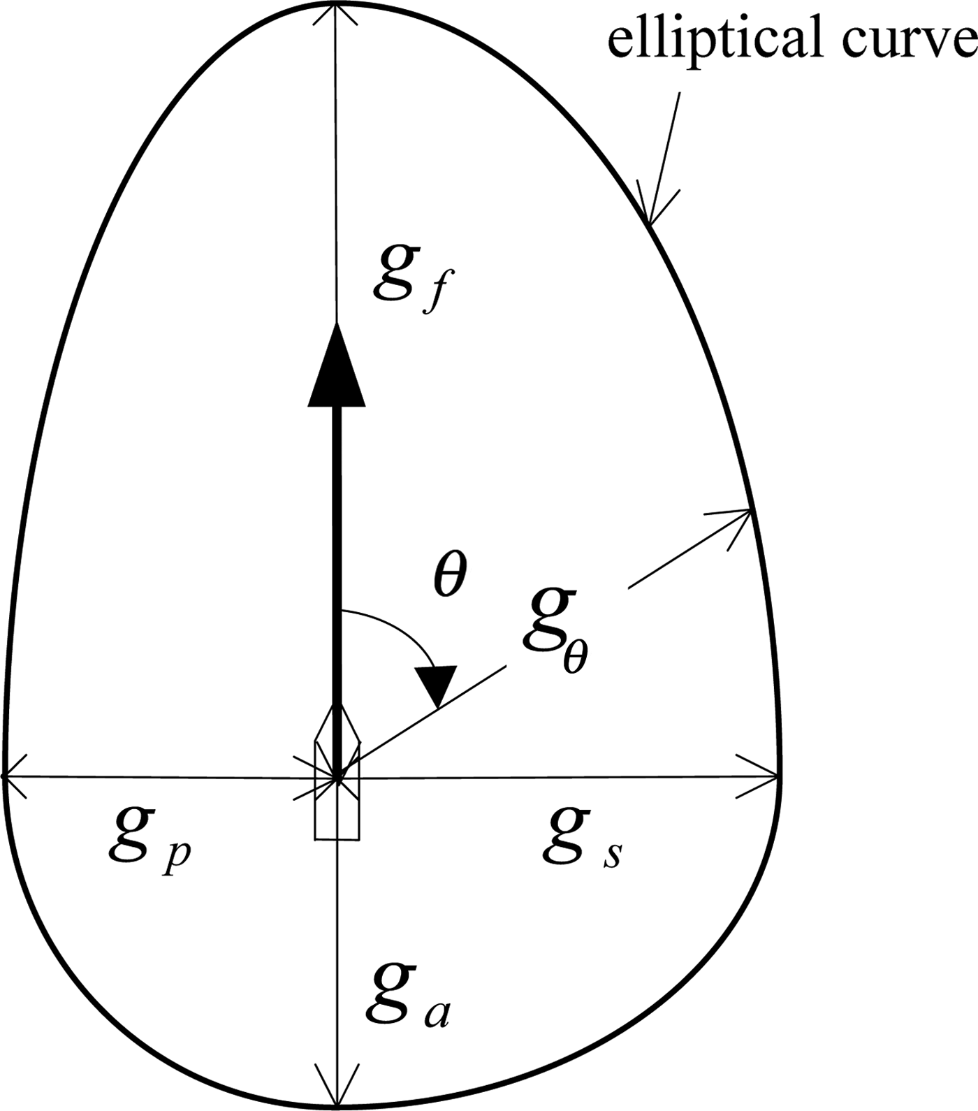
Further, assuming the speed function is governed by an elliptical form as seen in Figure 3, the speed in any given heading θ, i.e., g θ (v) and in short, g θ will be
 $$g_\theta = \displaystyle{{\left[ {\left( {1 + m} \right)g_f + \left( {1 - m} \right)g_a} \right] \cdot \left[ {\left( {1 + n} \right)g_s + \left( {1 - n} \right)g_p} \right]} \over {2\sqrt {\left[ {\left( {1 + m} \right)g_f \sin \theta + \left( {1 - m} \right)g_a \sin \theta} \right]^2 + \left[ {\left( {1 + n} \right)g_s \cos \theta + \left( {1 - n} \right)g_p \cos \theta} \right]^2}}} $$
where m and n are defined as
 $$m = \left\{ {\matrix{\;\;\;1, &{\hskip-39pt} {\theta \in \left[ { - \pi /2,\pi /2} \right)} \cr { - 1}, & {\theta \in \left[ { - \pi , - \pi /2} \right)\mathop \cup \left[ {\pi /2,\pi } \right)} \cr } } \right.$$
 $$n = \left\{ {\matrix{ \;\;\;1, & {\hskip-8pt}{\theta \in \left[ {0,\pi } \right)} \cr { - 1}, & {\theta \in \left[ { - \pi ,0} \right)} \cr } } \right.$$
Figure 3. Illustration of four directions of speed functions.
2.2. Calibration of Ship Domain Model
2.2.1. Iterative Calibration Process
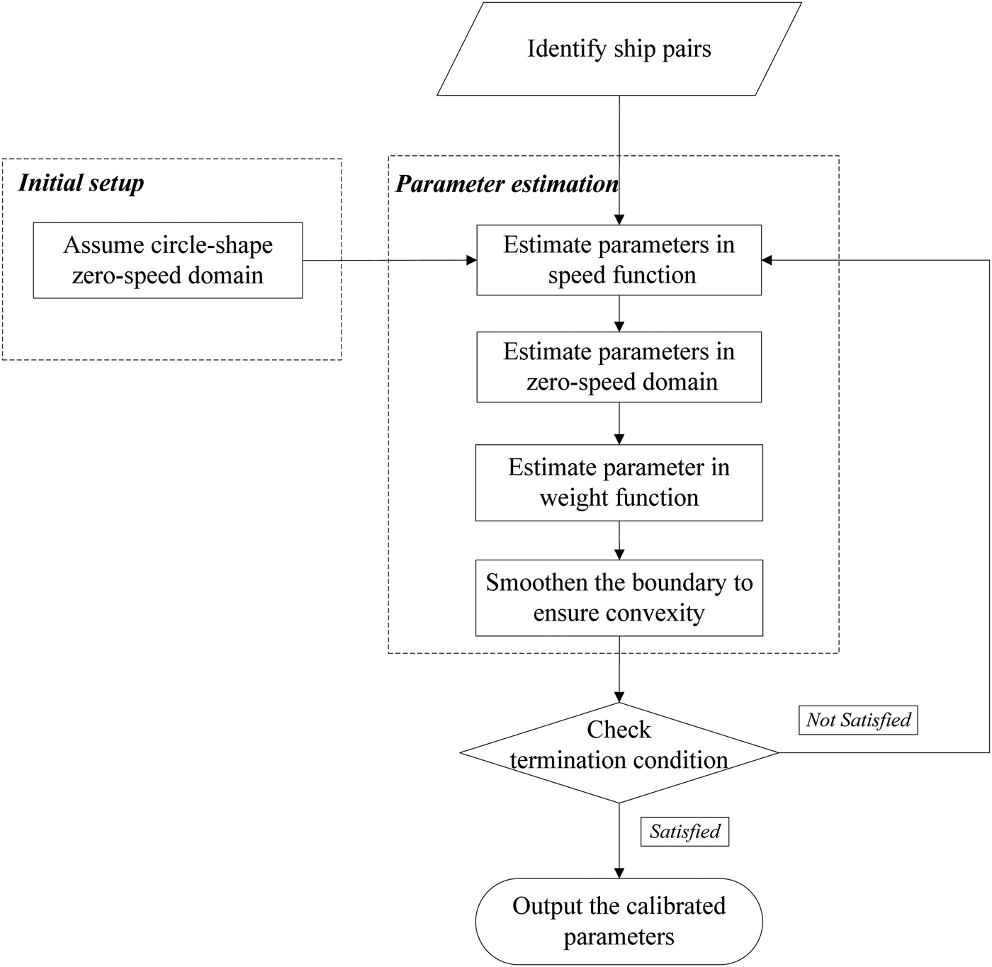
Due to the high degree of inter-relationships between the ship domain model and the speed function as well as the statistical uncertainties inherent in the data, it is difficult to derive a close-form solution of the parameter set. To determine the parameter values of the zero-speed domain model and the speed function, an iterative calibration procedure is adopted. The structure of the procedure is given in a flow chart shown in Figure 4. For the two sets of interrelated parameters in the ship domain model, at least one set of parameters needs to be assumed to start the interactive process. For convenience, taking the idea of the swinging circle of a ship anchoring position, a circular zero-speed domain of size L, i.e., α θ = 1, ∀i is initially assumed. Then the parameters in the speed function are determined, followed by an estimation of the weight function and a re-computation of the zero-speed domain. Since it is a free-form polygonal shape, non-convexity may exist at the boundary of the ship domain. In order to avoid potential fluctuation in using the ship domain, a step of smoothing the boundary of the ship domain is developed to ensure the zero-speed domain is convex. With the re-computed ship domain model, each ship-pair encounter needs to be reassessed to ascertain how likely the ship pair is to have a close encounter, resulting in possibly a new set of parameter values of the speed function as well as the ship domain. This procedure is iterated until convergence in the parameter values is achieved.
Figure 4. Flow chart showing calibration procedure of ship domain model.
2.2.2. Method for Estimating Parameters
The calibration procedure is set as an optimisation problem, with the parameters estimated by optimising the distance between the model behaviour and the extracted close encounters data. This is formulated as
 $$\eqalign{& Minimize \quad Fn\left( {{\alpha _k},\; {\lambda _x},\; {\mu _x}} \right) \cr & Subject \; to \cr &\quad \quad \quad \quad \quad \quad \quad\;\; {\alpha _k} \gt 0 \cr & \quad \quad \quad \quad \quad {\lambda _x} + 2{\mu _x}{v_{max}} \gt 0 \cr & \quad \quad \quad \qquad \qquad\;\; {\lambda _x} \gt 0 \cr & \quad \quad \quad \quad \quad \quad \quad\;\; {\mu _x} \gt 0} $$
where Fn stands for the objective function of the optimisation problem involving two sets of parameters; α k (k = 1, 2, … , 2π/Δ) are a set of parameters governing the zero-speed domain, and Δ is the angular discretization interval; λ x and μ x are the parameters in the speed function in which x = f, a, p, s representing the fore, aft, port and starboard side; v max is the maximum achievable speed. While the speed function is assumed to follow the quadratic form, it is necessary to constrain the parameters to the maximum v max so that only the monotonically increasing portion of the quadratic curve is used.
The optimisation function essentially seeks to minimise the errors between the safe distances obtained from the ship domain models and the observed values. The relative error function adopted is given by
 $$E_{rel} = \displaystyle{{\left\vert E \right\vert} \over d} = \displaystyle{{\left\vert {d - SD_{OS} - SD_{TS}} \right\vert} \over d}$$
where E is the estimation error, d is the observed distance between the two ships and SD OS and SD TS are the lengths of the domains in the direction of line of sight based on the relative bearing and heading of the two ships.
Among all the ship pairs, it is not known, a priori whether a particular pair in close range is necessarily in close encounter. Including all possible data pairs would make the calibration procedure tedious and superfluous, so some form of data reduction is necessary. In general, ships nearer the subject ship, i.e., OS, are more likely to be in close encounter and hence there is a higher probability that the space separation between the two ships will be governed by the ship domains to be modelled. This probability will decrease with larger space separation, vanishing quickly with the distance apart. Therefore, a weight function (w(E)) is defined in Equation (8) to account for the contribution of each ship pair data, and favour the ship pairs in close encounters. Since a larger E may be a result of lower likelihood of the ships being in close encounter, a modified exponential function is applied as
 $$w\left( E \right) = \left\{ {\matrix{e^{ - \omega E}, & E \ge 0 \cr {\hskip-17pt}1, & E \lt 0}} \right.$$
in which ω is the parameter of the exponential function. The objective function to be minimised is thus defined as the sum of the weighted relative error for each encounter, i.e.,
 $$Fn = \sum E_{rel} \cdot w\left( E \right)$$
The optimisation problem is solved using the Genetic Algorithm (GA) technique. The implementation of GA in this research is coded under the programming environment of MATLAB. The Global Optimisation toolbox in MATLAB provides various optimisation techniques including GA and it supports algorithmic customisation for users' purposes. For instance, the user can create a custom generic algorithm variant by modifying initial population and fitness scaling options or by defining parent selection, crossover, and mutation operators (MathWorks, 2012).
3. DATASET
3.1. Background
For the purposes of this paper, vessel movement data in Singapore Port and Singapore Strait were obtained from the Vessel Traffic Information System (VTIS) database operated by the Maritime and Port Authority of Singapore (MPA). A chart of Singapore VTIS coverage (known as STRAITREP operation areas) from the MPA website is shown in Figure 5 including Singapore Strait (Sector 7, Sector 8 and Sector 9) and Singapore Port. Seven hours of vessel movements covering both day and night conditions, at scan intervals of every 2 seconds were used. The data include the coordinate position, recorded speed and heading of each vessel tracked as well as the ship attributes, i.e., ship LOA, height, draft, Gross Tonnage (GT) and the Maritime Mobile Service Identity (MMSI) number.
Figure 5. Map of Singapore VTIS coverage including Singapore Strait and Port.
3.2. Data Preparation
To extract only relevant and useful information for analysis, some vessels captured under the VTIS were excluded. These include vessels that are anchored or moored, ships under special missions that may not follow the typical navigational rules, such as tug boats, police patrols and bunkering vessels as well as ships without an MMSI number such as fishing vessels and yachts.
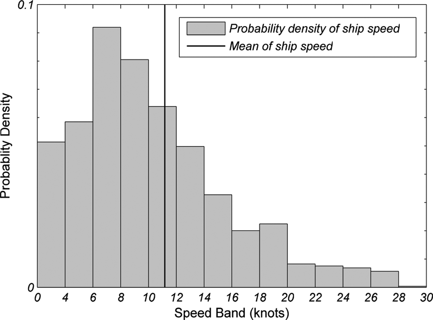
Following the data reduction process, a total of 624 vessels were captured during the survey period. Of these about 66% of the ships have LOA ranging from 50 m to 200 m with the longest ship up to 400 m. Tracking their positions throughout their movement within the study area, a total of around 2·7 million ship positions were obtained. Of these 57% are recorded in day time conditions (from 10:00 AM to 2:00 PM). The distribution of speeds of these vessels throughout their movement in the port is plotted in Figure 6. The wide variation of speeds should allow a good calibration study of the navigational behaviour. Based on the ship positions, 264,975 ship pairs have been identified for day time condition within a circular range with 2 nm radius. These ship pairs will seed the process of domain calibration with an initial dataset as indicated in Figure 4.
Figure 6. Probability density plot of ship speed.
4. RESULTS OF CALIBRATING SHIP DOMAIN MODEL
Normalising the ship domains with the ship LOA and at zero-speed, we obtain a calibrated non-dimensional ship domain which is independent of the LOA as well as ship speed as shown in Figure 7 along with the calibrated speed functions in Figure 8 for the four major sides, i.e., the fore, aft, port and starboard sides as illustrated in Figure 3 which will be used to scale up the normalised ship domain.
Figure 7. Non-dimensional ship domains at zero speed and 15 knots.
Figure 8. Speed functions at the four sides.
From Figure 7, the zero-speed domain is relatively circular in shape although the fore side of the zero-speed domain is obviously larger than the aft side, the starboard side and port side. Figure 8 shows that the domain enlarges significantly on the fore and aft sides with increasing speed while it enlarges marginally on the port and starboard sides. The value of the speed function on the fore side is consistently higher than that on the aft side at all speeds and it reaches 7·2 at 30 knots on the fore side compared 5·9 on the aft side. The values of speed function on the port and starboard sides are around 3·0 at the speed of 30 knots though it is slightly higher on the starboard side than that on the port side for all speeds. The enlargement of ship domain due to increased ship speed is shown in Figure 7 where the non-dimensional ship domains at the speeds of 0 knots and 15 knots are depicted. These results suggest that navigators are comparatively more sensitive to ships from the fore and aft directions than those approaching from the port and starboard sides, and more sensitive to ships in front than those going after it. It may be also inferred that the own ship is more likely to give way to ships from the starboard sides than those coming from the port sides.
5. DISCUSSION
This section aims to examine the usefulness of the proposed ship domain model in this paper to model safe spacing between moving ships. It is first achieved by evaluating the fitness of ship domains in representing real navigational behaviour inferred from traffic movement data. The proposed model in this paper and selected existing models of ship domain are considered. Using several case scenarios, the safe spacing developed in the proposed model in this paper is further compared with that derived from domain models in some earlier studies. This involves a systematic comparison of the shape and size taking into account factors such as ship heading and relative bearing, as well as whether the domain is around OS or TS.
5.1. Comparison of Models of Ship Domain Based on Proportion of Encroachment
There are a number of empirically-derived ship domains that have been previously studied. For the purpose of this comparison, two elliptical domains invariant with ship speeds developed by Fujii and Tanaka (Reference Fujii and Tanaka1971) and Coldwell (Reference Coldwell1983) will be used for the comparison with our proposed model. Based on data of overtaking encounters in Japanese waters, Fujii and Tanaka (Reference Fujii and Tanaka1971) assumed the magnitude of major and minor semi-axis of the ellipse (r and s respectively) to be proportional to the ship length, i.e., r = 7L and s = 3L. On the other hand, Coldwell (Reference Coldwell1983) found r = 6 cables and s = 1·75 cables.
The comparison of the different safe spacing kept is made on the basis of the amount of encroachment observed from the VTIS data. Encroachments are instances in which ships are in closer proximity than predicted by ship domain. If the ship domain is assumed correct, i.e., the critical encounter is when d = SD, then the number of encroachments, i.e., when d < SD, possibly represents the error associated with over-estimating the ship domain. On the other hand, if a deterministic ship domain is assumed, then ships found to lie beyond the predicted ship domain, i.e., d ⪆ SD may represent some form of under-estimation, although it may be argued that ships are not always at the critical position. Hence the true domain will be in a region where the error of over-estimation is minimal and where the error of under-estimation is rapidly rising.
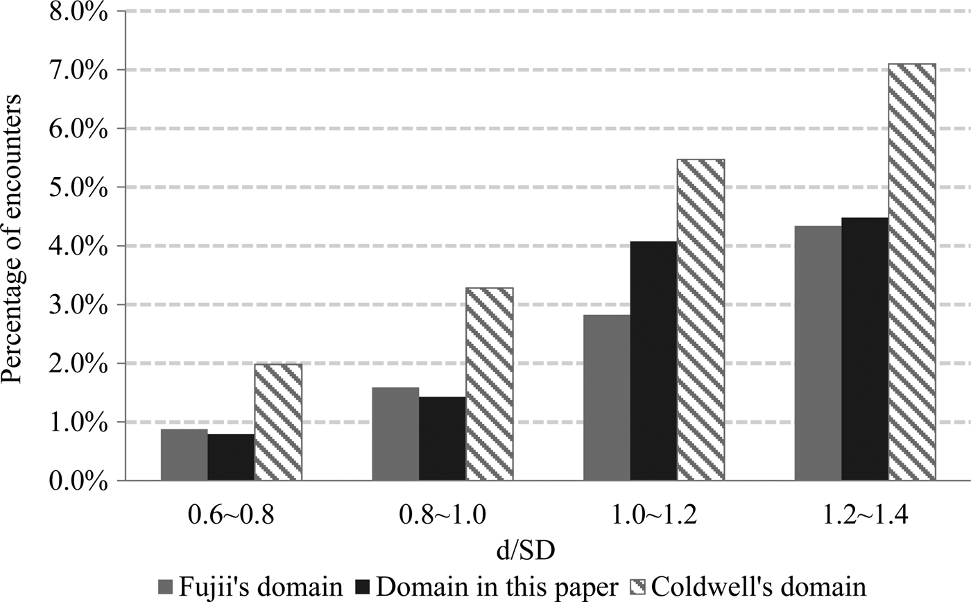
The errors of under-estimation or over-estimation of the safe spacing between ships modelled by the proposed ship models are compared with those generated by Fujii's models and Coldwell's models. The ratio of the actual distance between the two ships to the required safe distance, denoted by d/SD is used for evaluation. The percentages of encounters with respect to increment values of d/SD for three different domain models are plotted in Figure 9.
Figure 9. Percentage of encounters in the vicinity of critical encounter.
A low percentage of encroaching encounters, i.e., where d < SD, implies the chance that the ship domain is less likely to be smaller than predicted while a high percentage of encounters falling just beyond the predicted domain represent a strong resistance for the ship domain to be larger. Figure 9 shows that Coldwell's model has been overestimated since the percentage of encounters below the predicted domain (d/SD < 1) is high. Clearly, of the three models, Coldwell has a larger and hence over-estimated domain. Compared to Fujii's domain, the proposed domain is slightly better in yielding a slightly smaller error of over-estimation. On the other hand, the proposed domain gives a higher percentage of encounters just beyond the predicted domain than Fujii's model, suggesting that it has a higher resistance to under-estimation than Fujii's model. Taken together, it may be said that the proposed model gives the best solution.
5.2. Comparison of Ship Domains using Case Studies
This section compares the safe distances from the proposed model of ship domain with those generated from selected earlier studies under a variety of scenarios. Most previous models employ a single domain to represent the safe distance between two ships whereas the proposed model employs two individual domains around both OS and TS; an equivalent single domain is used to represent the safe distance from the proposed model. Some models only consider ship LOA and/or speed of a single ship, either OS or TS; the proposed model in this paper considers attributes of both OS and TS, a scenario involving a moving ship and a stationary ship is used to ensure compatibility in comparison.
5.2.1. Comparison with Circular-Type Domain
The safe distance from the proposed ship model is first compared with that of the circular-type model developed by Goodwin (Reference Goodwin1975) which has three unequal sectors with different radii, but are invariant with the ship speed and length. Since Goodwin's model is developed for single ship, a basic situation of a moving OS and stationary TS is examined under two scenarios: (1) a smaller and slower OS and (2) a larger and faster OS shown in Table 1.
Table 1. Ship attributes of OS and TS in comparison with Goodwin's model.

Note: TS is stationary therefore no heading for TS.
As shown in Figure 10, the safe distance based on the proposed model of a moving OS and stationary TS is superimposed on Goodwin's model for the two scenarios. There are clearly distinctive differences between the proposed model and Goodwin's model. Goodwin's model oversimplifies the safe spacing with large discontinuities at the sector boundaries. In addition, compared to the proposed model, Goodwin's model overestimates the safe distance, particularly on the port and starboard sides. This is partly because Goodwin's model is suitable for open seas (Zhao et al., Reference Zhao, Wu and Wang1993). There is however, closer similarity along the longitudinal axis. Nevertheless, since Goodwin's model does not account for the size of the ships and the speeds, there is a closer match between the proposed model and Goodwin's model on the aft side for the smaller and slower OS and on the fore side for the larger and faster OS. It may be argued that these are closer to the critical conditions in less restricted waters.
Figure 10. Comparison of safe spacing between proposed model and Goodwin's models.
Compared to Goodwin's model, the proposed model may be advantageous since it takes into account the ship size and dynamic effects. In addition, the comparison also implies that Goodwin's model is suitable for large and fast vessels because the vessels observed by Goodwin were large and medium ships (Zhao et al., Reference Zhao, Wu and Wang1993).
5.2.2. Comparison with Elliptical-Type Domains
Two elliptical-type domains are evaluated in this section – Coldwell's model (Coldwell, Reference Coldwell1983) which is developed around the OS and Fujii's model which is built around the TS. Both of the models are dependent on the ship LOA but independent of its speed.
Comparison with Coldwell's model is based on two scenarios representing two speed conditions of a large OS and a stationary TS as shown in Table 2. Figure 11 shows the comparison between Coldwell's model and the proposed model for the two scenarios in a head-on encounter of OS with LOA = 200 m and speeds of 15 and 20 knots. The comparison shows that the proposed model is reasonably compatible with Coldwell's model on the fore side but rather different on the starboard and port side. It should be noted that to account for the influence of general navigational rules on navigators' behaviour, i.e., to pass on the port side instead of the starboard side in head-on encounter, the safe spacing of Coldwell's model on the starboard side is larger than that on the port side. However, the preference to pass on the port side may not be equated to navigators having a lower tolerance of separation on the port side than the starboard side, especially in the empirical domain model developed from real navigational data.
Figure 11. Comparison of safe spacing between proposed model and Coldwell's model.
Table 2. Ship attributes of OS and TS in comparison with Coldwell's model.

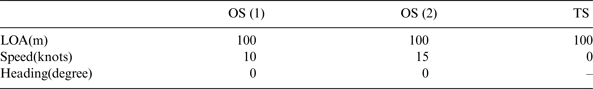
The comparison with Fujii's model (Fujii and Tanaka, Reference Fujii and Tanaka1971) is based on three scenarios with a moving OS of LOA = 100 m at speeds of 10 knots and 15 knots and a stationary TS of LOA = 100 m as tabulated in Table 3. The result of safe spacing from the two models is shown in Figure 12 and it can be seen that the proposed model with the same ship dimensions of OS and TS in scenario 1 approximately matches with Fujii's model although predicting slightly larger lateral sides and fore side and slightly smaller aft side. Furthermore, with a faster OS in scenario 2, the proposed model has been enlarged substantially on the fore and aft sides; it then has matched quite well with Fujii's model on the aft side.
Figure 12. Comparison of safe spacing between Fujii's model and proposed model.
Table 3. Ship attributes of OS and TS in comparison with Fujii's model.
Clearly the proposed model has a higher degree of freedom in the domain shape, e.g., by allowing different sizes on the fore and aft side, compared to the symmetrical elliptical domain which is constrained by the axial diameters. Consequently, the calibrated free-form domain model may give a better representation of reality than the constrained elliptical domain model. Moreover, the enlarged domain due to faster ship speed in the proposed model also suggests that Fujii's model, unlike the proposed model, is unable to account for the effect of the ship speed. Quite naturally, with a higher speed, the OS will require a larger separation from the TS and vice versa for a lower speed. This highlights the superiority of the proposed model that is sensitive to the ship speed.
5.2.3. Comparison with Polygonal-Type Domains
Based on the input from experienced navigators in a desktop calibration, Pietrzykowski and Uriasz (Reference Pietrzykowski and Uriasz2009) developed a polygonal model suitable in open sea for a specific pair of moving ships, in which both the ship length and speeds are considered.
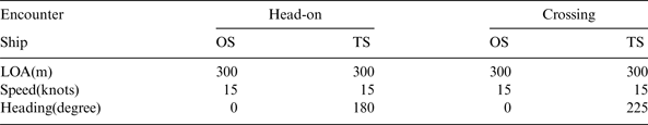
Pietrzykowski's model uses a 24-sided polygon and a fuzzy function to reflect the level of navigational safety, denoting this by γ ∈ [0, 1] where γ = 0 represents the very safe situation and γ = 1 represents the very dangerous situation (collision). For the purpose of comparison, two specific encounters, i.e., a head-on encounter and a crossing encounter with the ship attributes shown in Table 4 are considered. The safe spacing generated by Pietrzykowski's model with three levels of danger represented by γ = 0·5, 0·8, 0·9, along with the predicted safe spacing of the proposed model are shown in Figure 13 and Figure 14 for the two encounters respectively.
Figure 13. Comparison of safe spacing between proposed model and Pietrzykowski's model in a head-on encounter.
Figure 14. Comparison of safe spacing between proposed model and Pietrzykowski's model in a crossing encounter.
Table 4. Ship attributes of two moving ships in comparison with Pietrzykowski's model.
The comparison shows that the safe spacing in Pietrzykowski's model for both the head-on and crossing encounters, under the dangerous situation with γ = 0·9 prior to any collision is much smaller than that of the proposed model, though the shape of the two models are about similar. The proposed model appears to match Pietrzykowski's model for the case with γ = 0·8 particularly on the fore side, the port and starboard sides. Thus it is very reasonable to assume that Pietrzykowski's model for open seas under a relatively critical condition (assumed to be γ = 0·8) may be close to the case of ship movements in restricted waters. It should be noted that for the aft side in both encounters, the proposed model is significantly larger than that of Pietrzykowski's model for γ = 0·8 and even for a more favourable condition of γ = 0·5. This is reasonable and may be attributable to the way the aft side of the domain is obtained in the two models. Pietrzykowski derived the model from navigators in a desktop exercise assuming a hypothetically static situation exists, while in fact, under a dynamic situation, such a critical situation may not be possible. For example, while it may be possible to put a limiting comfortable space separation between two ships that are moving away from each other in opposite directions, such a critical situation is practically impossible and hence never observed. As the proposed model is calibrated using actual encounters rather than a desktop input, the lower likelihood of such critical encounters will also mean a lack of empirical data to justify a smaller domain under this situation. This may also explain why most empirical models (Coldwell, Reference Coldwell1983; Fujii and Tanaka, Reference Fujii and Tanaka1971) as shown in Figure 11 and Figure 12 generally have a much larger aft side than the port and starboard sides. This discussion further demonstrates that the proposed model is well developed empirically.
Summarising, there is generally good compatibility between the proposed model and Pietrzykowski's model, suggesting that the consideration of ship length and speed as well as the encounter type in this paper is suitable. In addition, the good match under the more dangerous situation of Pietrzykowski, particularly on the fore side, port side and starboard side provides good justification for the suitability of proposing a domain model that takes into account the encounter type of the ships.
Summarising the foregoing discussions on the comparisons of safe spacing generated by the proposed model with that from the previous models, it may be concluded that on the whole, the proposed model is compatible with other models particularly in the overall shape and on the fore and lateral sides. However, given that the proposed model accounts for different ship sizes and ship speeds as well as the different encounter types between ships, the proposed model that is developed for confined waters can be regarded as superior and more versatile than the models from previous studies. It is potentially more useful in examining ship separation under dynamically changing encounters and operating conditions.
6. CONCLUSIONS
Literature reviews have shown significant variation in the shape of existing ship domain models. The statistical methods for determining ship domains are also limited due to insufficient dataset, difficulties in separating the factors affecting the domain shape and size as well as unclear definitions. Few ship domain models have been developed for confined waters and the existing poor definitions and modelling of ship encounters may also restrict these empirical ship domains from broader applications. This paper shows that the proposed free-form empirical domain in confined waters can be modelled under a variety of operating conditions and navigational situations. By enforcing two individual domains of an asymmetrical polygonal shape around the OS and TS, the ship domain hence configured is able to provide the required safe distance for any encounter with changing relative bearing and heading. By innovatively employing a weight function, the iterative approach for calibrating the ship domain using vessel movements in Singapore Strait and Singapore Port has demonstrated reasonable results of ship domains. The superiority of the proposed model is demonstrated when compared with existing ship domain models, in that it presents better fitness to the movement dataset compared to Fujii's model and Coldwell's model.
The methodology used in calibrating the ship domain has great potential in mining trajectory data to study ship navigation. Further work to consider ship trajectories under day and night conditions and the effect of site and channel geometric constraints will allow a further refinement of the ship domain under the influence of other factors.
ACKNOWLEDGEMENTS
The authors are grateful to the Maritime and Port Authority of Singapore for the data and support in the study. The authors would like to extend special thanks to Capt. Mark Heah for the significant contribution and fruitful suggestion to this paper.