


Introduction
Ice shelves fringe around half of the continent of Antarctica. They present a crucial interface between ice sheet, ocean and atmosphere, and serve to regulate the rate at which grounded ice is lost to the ocean, making it essential to understand their ongoing evolution (Dupont & Alley Reference Dupont and Alley2005, Solomon et al. Reference Solomon, Qin, Manning, Chen, Marquis, Averyt, Tignor and Miller2007). Ice shelves are subject to melt and accumulation from both above and below, and generally evolve slowly through these processes (Pollard & DeConto Reference Pollard and DeConto2009, Pritchard et al. Reference Pritchard, Ligtenberg, Fricker, Vaughan, van den Broeke and Padman2012). However, they are also susceptible to abrupt collapse which can rapidly reduce the buttressing effect they provide and lead to significant and long-lived draw-down of grounded ice to the oceans (Scambos et al. Reference Scambos, Hulbe, Fahnestock and Bohlander2000, Gagliardini et al. Reference Gagliardini, Durand, Zwinger, Hindmarsh and Le Meur2010, Rott et al. Reference Rott, Müller, Nagler and Floricioiu2011, Berthier et al. Reference Berthier, Scambos and Shuman2012). Several instances of ice shelf disintegration have been observed around the Antarctic Peninsula in recent decades (Cook & Vaughan Reference Cook and Vaughan2010) but a comprehensive explanation for these events remains elusive (Glasser et al. Reference Glasser and Scambos2008).
A common precursor to abrupt ice shelf loss is unusually intense, extensive or prolonged surface melt and the presence of standing bodies of surface meltwater (melt ponds) (Scambos et al. Reference Scambos, Hulbe, Fahnestock and Bohlander2000, Sergienko & MacAyeal Reference Sergienko and MacAyeal2005, Van den Broeke Reference Van den Broeke2005). The extra hydrostatic pressure exerted by melt ponds may be sufficient to drive existing fractures completely through the full ice thickness by the process of hydrofracture, thereby irrevocably weakening the ice shelf (Van den Broeke Reference Van den Broeke2005, Luckman et al. Reference Luckman, Jansen, Kulessa, King, Sammonds and Benn2012, McGrath et al. Reference McGrath, Steffen, Rajaram, Scambos, Abdalati and Rignot2012). Two further mechanisms may serve to enhance the link between melt, ponding and collapse. First, where surface melting is common or prolonged, meltwater may percolate into the firn leading to densification, eventually to the point where firn air content approaches zero and no further infiltration is possible (Holland et al. Reference Holland, Corr, Pritchard, Vaughan, Arthern, Jenkins and Tedesco2011, Kuipers Munneke et al. Reference Kuipers Munneke, Ligtenberg, van den Broeke and Vaughan2014). This process transfers heat to deeper layers as water refreezes in the much colder firn (Vaughan Reference Vaughan2008), potentially affecting ice shelf dynamics and the fracture toughness because both are strongly dependent on ice temperature and its variation with depth (Rist et al. Reference Rist, Sammonds, Oerter and Doake2002, Jansen et al. Reference Jansen, Kulessa, Sammonds, Luckman, King and Glasser2010, Khazendar et al. Reference Khazendar, Rignot and Larour2011). A shelf made denser by frequent or long-term surface melt will be more capable of generating and sustaining melt ponds at the surface, but may be more resistant to fracture because of its higher mean temperature. Second, tensile flexure stresses exerted by hydrostatic rebound as melt ponds drain may further increase the likelihood of subsequent collapse (MacAyeal & Sergienko Reference MacAyeal and Sergienko2013, Banwell et al. unpublished). Therefore, a better understanding of the meteorology of ice shelves, of the extent and duration of surface melt, and of the formation and nature of melt ponds is desirable.
Following the collapse of Larsen A and B ice shelves in 1995 and 2002, respectively (Rott et al. Reference Rott, Skvarca and Nagler1996, Rack & Rott Reference Rack and Rott2004), the future development of their much larger and southerly neighbour, Larsen C, was of particular interest (Jansen et al. Reference Jansen, Kulessa, Sammonds, Luckman, King and Glasser2010). Larsen C Ice Shelf intersects the mean annual -9°C atmospheric isotherm, hypothesized to be the climatic limit of ice shelf viability (Morris & Vaughan Reference Morris and Vaughan2003), a limit that is rapidly moving south with the exceptional climatic warming experienced along the Antarctica Peninsula (Turner et al. Reference Turner, Colwell, Marshall, Lachlan-Cope, Carleton, Jones, Lagun, Reid and Iagovkina2005, Reference Turner, Barrand and Bracegirdle2013, Vaughan Reference Vaughan2006, Monaghan et al. Reference Monaghan, Bromwich, Chapman and Comiso2008). The northern part of this ice shelf is also known to be approaching the level of densification that preceded the collapse of Larsen B Ice Shelf (Holland et al. Reference Holland, Corr, Pritchard, Vaughan, Arthern, Jenkins and Tedesco2011) and melt ponds are commonly reported. Therefore, Larsen C Ice Shelf is of particular interest for understanding the processes of surface melt and pond formation, and may provide an example of how ice shelves elsewhere will respond to atmospheric warming in the future.
To the east of the Antarctic Peninsula, low-level atmospheric conditions are commonly cooler than to the west, being strongly influenced by equator-ward winds bringing cold air from the Antarctic continent. During periods of westerly flow across the Antarctic Peninsula, warm, dry downslope winds, known as föhn winds, blow over Larsen C Ice Shelf. Although originally pertaining exclusively to the Alps, the term ‘föhn’ has become an umbrella term for warm, dry downslope winds anywhere on earth, although regional terms such as the Chinook or Santa Ana in North America remain popular. The warm, dry signature of föhn winds is a result of the sourcing of air from aloft, and/or the diabatic heating and drying of air as it ascends and passes over mountains (Whiteman Reference Whiteman2000, Elvidge et al. Reference Elvidge, Renfrew, King, Orr, Lachlan-Cope, Weeks and Gray2014). Föhn winds are able to ‘flush away’ any pool of cool air resident above Larsen C Ice Shelf, bringing warm air to near-surface level (King et al. Reference King, Lachlan-Cope, Ladkin and Weiss2008, Munneke et al. Reference Munneke, van den Broeke, King, Gray and Reijmer2012), and have been found to be associated with exceptionally high melt rates on the ice shelf. Munneke et al. (Reference Munneke, van den Broeke, King, Gray and Reijmer2012) used surface observations and a surface energy budget model to investigate a case in 2010 of westerly summer föhn across the Antarctic Peninsula. The residual energy available for melting was found to surpass 100 Wm-2 during föhn days (Munneke et al. Reference Munneke, van den Broeke, King, Gray and Reijmer2012). These large values were a result of large downward fluxes of shortwave radiation as a result of the dry, cloudless leeside föhn conditions, and sensible heat due to the warmth of the föhn air. Föhn-influenced surface melt is also seen in the Dry Valleys of East Antarctica (Speirs et al. Reference Speirs, McGowan, Steinhoff and Bromwich2013). Recent research has shown that stronger circumpolar westerlies associated with the shift towards an increasingly positive phase of Southern Annular Mode (SAM; the major mode of climate variability in the southern hemisphere) over the past c. 50 years are probably enhancing the frequency and/or amplitude of föhn warming events to the eastern flank of the Antarctic Peninsula (Orr et al. Reference Orr, Cresswell, Marshall, Hunt, Sommeria, Wang and Light2004, Marshall et al. Reference Marshall, Orr, van Lipzig and King2006, Turner et al. Reference Turner, Barrand and Bracegirdle2013).
In this study, a novel remote sensing approach was used to assess the nature of surface melt on Larsen C Ice Shelf and meteorological modelling was used to explain the observed spatio-temporal pattern of melt in terms of föhn events. Methods for monitoring melt pond development in the future were also explored.
Methods
Surface melt detection
Surface melt on large ice bodies from ice sheets to ice shelves is most effectively measured using satellite microwave instruments. This is due to the necessity for the daily or near-daily imaging provided by cloud-independent microwave instruments, the synoptic overview presented by satellites, and the high sensitivity of microwave radiation to the presence of liquid water at or near the Earth surface (Stiles & Ulaby Reference Stiles and Ulaby1980, Ulaby & Stiles Reference Ulaby and Stiles1981, Kunz & Long Reference Kunz and Long2006, Tedesco & Monaghan Reference Tedesco and Monaghan2009). However, previous studies have been limited in spatial resolution to several km for scatterometer data (e.g. Nghiem et al. Reference Nghiem, Steffen, Kwok and Tsai2001, Steffen et al. Reference Steffen, Nghiem, Huff and Neumann2004, Trusel et al. Reference Trusel, Frey and Das2012, Barrand et al. Reference Barrand, Vaughan, Steiner, Tedesco, Munneke, van den Broeke and Hosking2013) or tens of km for passive microwave sensing (e.g. Ridley Reference Ridley1993, Fahnestock et al. Reference Fahnestock, Abdalati and Shuman2002, Torinesi et al. Reference Torinesi, Fily and Genthon2003, Picard et al. Reference Picard, Fily and Gallee2007, Tedesco Reference Tedesco2009, Tedesco & Monaghan Reference Tedesco and Monaghan2009), thus a very detailed examination of melt patterns has not hitherto been achieved.
Synthetic aperture radar (SAR), a satellite active microwave imaging method capable of acquiring data at a much higher spatial resolution than scatterometer or radiometer, has not previously been used for snow melt detection because the high spatial resolution normally precludes a sufficient temporal sampling rate. However, the European Space Agency’s (ESA) Envisat Advanced SAR (ASAR) was equipped with an imaging mode capable of achieving high spatial resolution and was operated in such a way as to acquire near daily repeat images at polar latitudes. The wide swath mode (WSM) has a nominal spatial resolution of 150 m and images from Larsen C Ice Shelf were acquired, albeit with a variety of view azimuth and mean incidence angles, on average every 2 days between late 2006 and the loss of the satellite in April 2012. The high sensitivity of C-band microwave backscatter to the transition between water in solid and liquid states (and thus, between frozen and melting conditions at the surface and near-surface) means that these data can be used in essentially the same way as Seawinds QuikSCAT Ku-band scatterometer data (e.g. Nghiem et al. Reference Nghiem, Steffen, Kwok and Tsai2001, Trusel et al. Reference Trusel, Frey and Das2012, Barrand et al. Reference Barrand, Vaughan, Steiner, Tedesco, Munneke, van den Broeke and Hosking2013), but at a much higher spatial resolution, to retrieve surface melt extent and duration from ice shelves for summers 2006–07 to 2011–12.
Liquid water absorbs microwave radiation very effectively (Ulaby et al. Reference Ulaby, Moore and Fung1986), therefore the onset of surface melt can be inferred by a significant drop in SAR backscatter. To eliminate the impact of variations in local topography and surface roughness, which also affect backscatter, the melt-induced reduction in backscatter was calculated relative to the mean value when the surface was frozen; the winter mean was calculated using all images from June, July and August. The drop-off in backscatter caused by melt is so steep that other variations in image radiometry resulting from the range of view azimuth and incidence angles presented by ASAR WSM data are not significant, and results are only weakly sensitive to the threshold used for melt detection. A threshold constant of 3 dB (or a 50% reduction in power) was chosen, consistent with previous studies (e.g. Ashcraft & Long Reference Ashcraft and Long2006, Wang et al. Reference Wang, Sharp, Rivard and Steffen2007, Trusel et al. Reference Trusel, Frey and Das2012, Barrand et al. Reference Barrand, Vaughan, Steiner, Tedesco, Munneke, van den Broeke and Hosking2013).
The full sequence of ASAR images was ortho-rectified to a common map projection (polar stereographic) using the National Snow and Ice Data Center (NSIDC) 1 km digital elevation model (Bamber et al. Reference Bamber, Gomez-Dans and Griggs2009) and the winter mean image derived. Each reprojected image was then classified on a pixel by pixel basis into melting or frozen depending on the backscatter value relative to the winter mean (> 3 dB below the winter mean equates to melting). Melting may refer either to snow that is actively undergoing the process of melting, or to liquid water within the snowpack from a previous melt that has not yet refrozen. From the sequence of classified images, summaries by pixel of melt-onset day, melt duration and freeze-onset day were derived as follows: melt onset was calculated as the day on which melt had been detected for a minimum of seven consecutive days, thereby mitigating against spurious low backscatter values due to speckle noise or short-lived melt events in the transition from winter to spring. Other studies (e.g. Tedesco Reference Tedesco2009, Barrand et al. Reference Barrand, Vaughan, Steiner, Tedesco, Munneke, van den Broeke and Hosking2013) have used three days but seven days was chosen to ensure that the transition was based on at least three images (mean imaging frequency is two days). Freeze onset was calculated in a similar manner but seeking seven consecutive days of non-melt conditions per pixel. Melt duration was calculated as the sum of days of melt detected, and thus does not necessarily correspond exactly to the numerical difference between these interpretations of melt-onset day and freeze-onset day. In all cases, melt state in each pixel on days for which no images were acquired were assumed to follow the most recent observation, while days for which more than one image were acquired were assigned according to the last image acquired on that day (when melt was most probably occurring).
Meteorological modelling
The UK Met Office Unified Model (MetUM) was used to investigate meteorological conditions on Larsen C Ice Shelf during the 2010–11 melt season. Version 7.6 of the MetUM was used, which employs a non-hydrostatic, fully compressible, deep atmosphere with a semi-implicit, semi-Lagrangian, predictor-corrector scheme to solve the equations of motion (Davies et al. Reference Davies, Cullen, Malcolm, Mawson, Staniforth, White and Wood2005). The model set up is as described in Orr et al. (Reference Orr, Phillips, Webster, Elvidge, Weeks, Hosking and Turner2013). Applying an objective criterion to measurements from an automatic weather station on Cole Peninsula (inland of the Larsen C grounding line) indicates that föhn conditions were seen for around 30% of the time between January and March 2011. To characterize the spatial nature of such föhn events, the study focuses on a single föhn event across the Antarctic Peninsula between 4 and 5 February. The MetUM 1.5 km model was used as a tool to examine the nature of the leeside response during a westerly föhn event over the Antarctic Peninsula. Elvidge et al. (Reference Elvidge, Renfrew, King, Orr, Lachlan-Cope, Weeks and Gray2014) demonstrate considerable skill using this model in the reproduction of föhn conditions when compared with aircraft observations.
The model is run with minimum horizontal grid spacing of 1.5 km, 70 vertical levels and a time step of 30 seconds. The MetUM 1.5 km model is nested within a coarser model with a horizontal grid spacing of 4 km (MetUM 4 km), and is initialized from MetUM 4 km output after 6 hours run-time. These models use high resolution daily sea ice and sea surface temperature fields derived from the Operational Sea Surface Temperature and Sea Ice Analysis (OSTIA) system (Stark et al. Reference Stark, Donlon, Martin and McCulloch2007). The MetUM 4 km model is, in turn, nested within a global model (25 km horizontal grid spacing), forced by Met Office operational analysis.
Surface pond identification
Satellite remote sensing has previously been used to detect and measure lakes or ponds on both ice sheets and sea ice (e.g. Selmes et al. Reference Selmes, Murray and James2011, Rösel Reference Rösel2013). In contrast, remote sensing of melt ponds on ice shelves has not attracted much attention. Since the size of such ponds are expected to be on the order of hundreds of metres to kilometres, and the fate of individual ponds is of interest, high spatial resolution sensors are required to detect and monitor them. Standing surface water would be expected to have a spectral signature distinct from surrounding firn and ice at visible wavelengths and also in the near-infrared (NIR) because water is strongly absorbent in this part of the spectrum (Rösel Reference Rösel2013). A pond which has frozen during or at the end of the melt season will be harder to discriminate in visible/NIR data not least because of its capacity to quickly become covered and hidden by snow. Using a different part of the electromagnetic spectrum, microwave backscatter from water bodies will vary significantly depending on whether the surface of the water is smooth (low backscatter) or rough through wind action (high backscatter). A frozen pond may be distinct in SAR data because it presents smooth surface scatterers in contrast to the surrounding volume scatterers in the firn (Kunz & Long Reference Kunz and Long2006), and fresh snow will be invisible at microwave wavelengths thus will not hide the ponds below.
Of all the high spatial resolution optical and microwave sensors available, Landsat, MODIS and Envisat ASAR WSM are the most likely to yield observations of melt ponds because of the large archives of data acquired in recent years presenting maximal temporal sampling, thus these were investigated further. All suitably cloud-free data from the Landsat archive (glovis.usgs.gov) were inspected online for the period 1990–2013 and a number of images in which melt ponds were visible were downloaded and resampled to the same projection as the ASAR WSM data. These were then explored as band 7-4-2 (shortwave-infrared, NIR, green) false-colour composites commonly used to discriminate ice surface features. All suitably cloud-free MODIS data were provided by NSIDC and each channel 2 (NIR) Larsen C Ice Shelf subset image was downloaded from the NSIDC website (nsidc.org/data/iceshelves_images/index_modis.html) and reprojected to the common grid. For the ASAR WSM data, the mean March backscatter for each available year were chosen, derived by taking the mean pixel value for all images acquired in March, because this avoids the potentially high backscatter variability from ponds and reduces the impact of speckle noise.
Results
Surface melt extent and duration
The use of Envisat ASAR WSM data allowed melt duration maps at a spatial resolution of 150 m to be derived for summers 2006–07 to 2011–12 (Fig. 1). The mean annual melt days between the six available melt seasons are also presented to illustrate the long-term pattern of melt.

Fig. 1 Annual surface melt duration on Larsen C Ice Shelf for the six melt years (August–July) for which Envisat wide swath mode (WSM) synthetic aperture radar (SAR) data are available. Note the retrieval of melt duration on small glaciers draining west into Marguerite Bay (bottom left of panels). For the three years of overlap in data availability, melt duration for the Antarctic Peninsula from Seawinds QuikSCAT is also shown (insets). The lowermost panel shows mean annual melt days from WSM for the entire six-year period. Colour denotes number of melt days per year; image brightness is the mean Envisat SAR (or QuikScat) backscatter for the observation period. Spatial resolution follows the WSM data (c. 150 m) or the QuikScat data (c. 5 km).
The quality of the melt duration maps produced were assessed by comparison to similar products derived from Seawinds QuikSCAT Ku-band microwave scatterometer data in years where data were available from both instruments (Fig. 1). The QuikSCAT data have been independently validated against surface observations and surface energy modelling results. The broad pattern of melt duration and absolute number of melt days showed no significant disparity between the two approaches giving confidence that the ASAR WSM data were suitable for assessing surface melt at a higher spatial resolution than previously possible. The comparison between approaches was not explored more quantitatively because the primary interest was in the spatial pattern of surface melt, rather than the absolute correspondence between melt duration derived by satellite and that experienced at the surface.
Several interesting features were observed in the new high spatial resolution maps. Melt duration was captured on relatively small glaciers draining the Antarctic Peninsula to the West, as well as on the ice shelf itself, suggesting that the improved spatial resolution makes this method also applicable to much smaller ice masses. Inter-annual variability in melt duration was apparent, as exemplified by the difference between summers 2007–08 (maximum melt) and 2009–10 (minimum melt) but the spatial pattern of melt was consistent from year to year and the six-year mean was a good indicator of the multi-annual geographical distribution. A decrease in melt duration on Larsen C Ice Shelf from north–south was apparent in every year of data acquisition, and this followed the expected decrease in mean air temperature with increasing latitude. Superimposed on this was a west–east decrease in melt duration.
Most notable was the high concentration of melt in Larsen C inlets where glaciers from the Antarctic Peninsula drained into the ice shelf. This concentration occurred in all years, was manifest as around double the number of melt days in inlets compared to elsewhere on the shelf, and southern inlets in particular showed much longer annual melt duration than the rest of the ice shelf at similar latitude. The distinctive pattern of melt in inlets was also apparent in the measured days of melt onset and freeze onset (Fig. 2). Earlier melt onset and later freeze onset associated with generally warmer conditions were seen towards the north of Larsen C Ice Shelf, where expected, but was also evident in the western inlets.
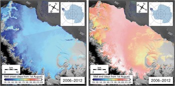
Fig. 2 Mean day of melt onset (left panel) and melt end (right panel) relative to 1 August for the observation period. Colour denotes day number; image brightness is the mean Envisat SAR backscatter for the observation period.
Föhn wind modelling
A westerly föhn event above Larsen C Ice Shelf occurred between 4 and 5 February 2011. This event was associated with relatively weak (<10 m s-1), strongly stratified approaching flow, and has previously been investigated using aircraft observations and MetUM simulations. Whilst much of the lower level flow was blocked and largely deflected northwards by the Antarctic Peninsula, some flow was able to pass over the Antarctic Peninsula, plunging down the lee slopes as föhn winds. Plan plots of wind velocity and temperature at 150 m above mean sea level at 10 UTC on 5 February 2011 are shown in Fig. 3, derived from the MetUM 1.5 km simulation. The model data have been linearly interpolated to the same domain used for melt duration plots. Strong westerly winds emerging from the major leeside inlets separated by regions of calmer flow are shown in Fig. 3a. The föhn warming effect is illustrated in Fig. 3b. A cross-Peninsula temperature gradient is apparent, with temperatures immediately to the west (upwind) of the Antarctic Peninsula being considerably lower than those immediately to the east (downwind). However, away from the base of the lee slopes above Larsen C, leeside temperatures fall considerably. This east–west temperature gradient is similar to that observed in annual melt durations. A comparison of Figs 1 & 3b reveals a strong resemblance between the distribution of simulated leeside temperatures during the event and the distribution of annual melt duration between 2006 and 2012.

Fig. 3 Plan (x-y) plots of a. wind speed and vectors, and b. temperature, at 150 m above mean sea level at 10 UTC on 5 February 2011 from the MetUM 1.5 km model, interpolated to the same domain used for melt duration plots. Major inlets are marked: CI=Cabinet Inlet, MI=Mill Inlet, WI=Whirlwind Inlet, MOI=Mobil Oil Inlet. Inset in b. shows the MetUM 4 km (red) and 1.5 km (blue) domains over Antarctic Peninsula orography.
Close to the base of the lee slopes the descending föhn penetrates to low levels, helping maintain a well-mixed boundary layer. Further east, re-ascent of the föhn flow and reduced turbulent mixing leads to a diminished föhn warming effect, explaining the west–east temperature gradient above Larsen C apparent in Fig. 3b. An intriguing characteristic of the leeside temperature field is that the warmest regions are not coincident with the strongest föhn winds (föhn jets), but with the regions of calmer flow in between the jets (Fig. 3).
Despite the cooler jets, surface sensible heating was considerably greater in the jets than in adjacent regions of calmer flow, according to the MetUM 1.5 km simulation. This was due to the stronger winds inducing greater turbulent heat exchange. Furthermore, föhn winds would be expected to penetrate to the surface more frequently and for longer periods within the inlets due to the positioning of mountain passes upslope of the inlets (promoting föhn winds via gap flows) and the convergence of downslope winds; therefore, greater and more frequent föhn-related melt within the inlets was expected. Given the sensitivity of melt rates to air temperature and wind speed, the pattern of the observed melt durations, with highest melt rates close to the Antarctic Peninsula’s easterly slopes, particularly within the inlets where föhn winds were greatest, were strongly explained by such föhn events.
Surface pond location and characteristics
There are insufficient archived cloud-free or microwave data from MODIS, Landsat and Envisat ASAR WSM to investigate multi-annual trends in size or distribution of melt ponds on Larsen C Ice Shelf. This appears to be because the data record is relatively short and increasingly sparse into the past, especially for sufficiently frequent SAR data, and Larsen C Ice Shelf is very often obscured by cloud in optical data. Therefore, only a small subset of available images in which melt ponds were observed are discussed in order to explore how melt ponds might be detected and monitored in future (Figs 4 & 5).

Fig. 4 Example MODIS channel 2 (near-infrared) image of Larsen C Ice Shelf (www.nsidc.org). Red box indicates Cabinet Inlet and shows extent of data presented in later figures. Dark patches within Cabinet Inlet and neighbouring inlets Adie (to the north) and Mill (to the south) are interpreted as water at or near the surface.

Fig. 5 Selection of example images of Cabinet Inlet illustrating the extent to which melt ponds may be discriminated in a variety of satellite images, and showing their size and distribution. a. MODIS channel 2 (near-infrared, NIR) images of Cabinet Inlet from summer 2002–03. b. MODIS channel 2 (NIR) images of Cabinet Inlet from summer 2006–07. c. Landsat false colour (bands 7-4-2) images of Cabinet Inlet (diagonal black stripes result from the scan line correction fault). d. ASAR March mean backscatter images from 2007, 2008 and 2009.
MODIS would be expected to be a good candidate for monitoring melt ponds because it has an appropriate spatial resolution in the red and NIR channels (250 m), and a suitable repeat imaging frequency (daily or better at polar latitudes). Figure 4 illustrates the best example of melt pond detection in MODIS data which exhibits much darker pixels where the water absorbs incident NIR radiation. Melt ponds are evident in Adie, Cabinet and Mill inlets. Further data from Cabinet Inlet alone illustrate how ponds appear in a wider variety of satellite data (Fig. 5). Nevertheless, similar images to those illustrated in Fig. 4 are rare either because melt ponds do not develop, or because predominant cloud cover prevents their detection. The latter explanation is more feasible because the temporal distribution of archived cloud-free images often has long gaps towards the end of the summer. The evolution of ponds in Cabinet Inlet in early 2003 is shown in Fig. 5a. At the end of January 2003 ponds were visible but ten days later they had all but disappeared. A similar three-week evolution of pond appearance and disappearance in 2007 is shown in Fig. 5b and in this case it is also possible (in the full resolution digital images) to detect the enlargement of the ponds between 31 December 2006 and 7 January 2007, suggesting rapid filling and/or flow of water across the ice shelf in periods of intense melt.
In more than three decades of acquisition of Landsat data, only a dozen images were found showing melt ponds on Larsen C Ice Shelf because, as well as the predominance of cloud cover, the imaging period is at best 16 days and data are not automatically acquired and archived as they are from MODIS. By way of example, images of melt ponds in Cabinet Inlet from 2004, 2006 and 2007 using false-colour composites are presented in Fig. 5c. The pattern of melt ponding (dark blue) corresponds to that seen in MODIS data but is presented at the higher spatial resolution of 30 m.
Melt ponds were generally discernible in individual Envisat ASAR WSM images from late summer, but these data were also subject to speckle noise, variable data coverage, incidence and view azimuth angles, and the same summer reduction in backscatter that were used to detect surface melt. Therefore, images of mean backscatter from March in each available year which overcome these limitations were chosen, and the derived images with three of the available six years of data were illustrated (Fig. 5d). Melt ponds were evident as patches of lower backscatter which were very similar year to year and match the patterns seen in the optical data. The reduced backscatter was attributed to the smoothness of the frozen pond surface in contrast to the surrounding firn (snowfall subsequent to pond freezing would not obscure the ponds in SAR data because cold fresh snow is essentially invisible at C-band).
Together the images shown in Fig. 5 illustrate that melt ponds in Cabinet Inlet were elongated in the east–west direction and were aligned with the flow direction. The spatial pattern of ponding was highly consistent from year to year and ponds ranged in size from tens of metres in width to tens of kilometres in length.
Discussion
The pattern of increasing surface melt duration, earlier melt onset, and later freeze onset from East–West on Larsen C Ice Shelf, and the high concentration of melt in the western ice shelf inlets may be explained by the föhn warming effect resulting from predominantly westerly winds (Munneke et al. Reference Munneke, van den Broeke, King, Gray and Reijmer2012, Barrand et al. Reference Barrand, Vaughan, Steiner, Tedesco, Munneke, van den Broeke and Hosking2013). A shift towards increasingly positive phase of SAM over the past c. 50 years has induced stronger circumpolar westerlies, enhancing the frequency and/or amplitude of föhn warming events to the east of the Antarctic Peninsula (Orr et al. Reference Orr, Cresswell, Marshall, Hunt, Sommeria, Wang and Light2004, Marshall et al. Reference Marshall, Orr, van Lipzig and King2006, Turner et al. Reference Turner, Barrand and Bracegirdle2013). The overall effect of föhn winds is to enhance leeside surface melt via enhanced surface solar radiation and sensible heat fluxes. The greatest föhn-induced melt should be expected to be close to the base of the Peninsula’s lee slopes due to greater near-surface air temperatures, and beneath föhn jets due to stronger near-surface winds and more frequent occurrences of föhn reaching the surface here. Note this is despite the jets being slightly cooler than adjacent calmer regions of föhn air; a result of lower, potentially cooler source altitudes for the föhn jets, which are the downwind continuation of gap winds across lower sections or ‘gaps’ in the Antarctic Peninsula’s crest (Elvidge et al. Reference Elvidge, Renfrew, King, Orr, Lachlan-Cope, Weeks and Gray2014). The distribution of leeside warming and winds evident in the case studied here qualitatively resembles that of another westerly föhn event over the Antarctic Peninsula a week earlier on 27–28 January 2011 (Elvidge et al. Reference Elvidge, Renfrew, King, Orr, Lachlan-Cope, Weeks and Gray2014). A stronger case of cross-Peninsula westerlies exhibits some significant differences in dynamics and leeside response, though the key elements of greatest temperatures at the foot of the lee slopes and strongest winds within the inlets are consistent (Elvidge et al. Reference Elvidge, Renfrew, King, Orr, Lachlan-Cope, Weeks and Gray2014).
The resulting gradient in surface melt explains, in turn, the pattern of ice shelf densification observed by Holland et al. (Reference Holland, Corr, Pritchard, Vaughan, Arthern, Jenkins and Tedesco2011) who showed a corresponding lower air content towards the north of Larsen C Ice Shelf and particularly in the north-western embayments including Cabinet Inlet. This part of the ice shelf is approaching the densification observed in Larsen B Ice Shelf immediately prior to its collapse (Holland et al. Reference Holland, Corr, Pritchard, Vaughan, Arthern, Jenkins and Tedesco2011), suggesting a possible link between föhn-enhanced surface melt and potentially unstable ice shelf conditions. Our observations of melt ponds are also spatially consistent with this focus in melt duration. Where surface melt is most concentrated the ice shelf has become most dense, and is most able to both generate and sustain melt ponds on the surface.
There are two possible hypotheses to explain the rapid disappearance of the melt ponds. The first is that they freeze over at the end of summer and rapidly become covered by snow which obscures them from optical satellite instruments. The second is that, in a similar way to melt lakes on the Greenland ice sheet, they drain through fractures in the ice shelf, possibly as a result of hydrofracture (e.g. Das et al. Reference Das, Joughin, Behn, Howat, King, Lizarralde and Bhatia2008). The ice in this part of the shelf has near-zero air content (Holland et al. Reference Holland, Corr, Pritchard, Vaughan, Arthern, Jenkins and Tedesco2011) and its dynamic regime is compressive (Jansen et al. Reference Jansen, Kulessa, Sammonds, Luckman, King and Glasser2010). This favours the first hypothesis because the melt ponds are observed in the SAR data at the end of summer. However, the alternative hypothesis cannot be completely ruled out. If near-zero air content is a pre-condition for ice shelf disintegration then the coincident melt ponds are already commonly present to provide a possible trigger for collapse (MacAyeal & Sergienko Reference MacAyeal and Sergienko2013), and there may already be fractures through the full ice thickness in response to hydrofracture. Future monitoring of ice shelf melt ponds is therefore highly desirable.
The investigations of Larsen C Ice Shelf show that melt ponds are observable in optical satellite data but the predominant cloud conditions and the potentially short window of opportunity to observe these ephemeral features means that an alternative method of monitoring them is required. Data from SAR of sufficient spatial resolution and temporal sampling frequency may be used to perform this role. The launch of ESA’s Sentinel 1 mission in 2014 may sufficiently extend the archive of suitable data to allow trends in melt pond generation to be explored in future. Melt ponds are observed up to tens of kilometres in length and are aligned with the flow direction suggesting that they congregate in surface depressions arising from ice flow and/or basal melt processes. Their size suggests that a reservoir of water can regularly form which may be sufficient to sustain the hydrofracture process, although further research is required on the small-scale topography of the inlets to properly characterize melt pond depth and volume.
In conclusion, using a novel source of satellite microwave imagery and meteorological modelling we have highlighted, and provided an explanation for, the concentration of surface melt and ponding on the western inlets of Larsen C Ice Shelf. This pattern of melt helps to account for the distribution of densification observed by Holland et al. (Reference Holland, Corr, Pritchard, Vaughan, Arthern, Jenkins and Tedesco2011) and highlights a potential contributing process to the collapse of ice shelves elsewhere.
Acknowledgements
Envisat SAR data was kindly provided by the European Space Agency (ESA Project AOCRY-2676) and collected in part by the Natural Environment Research Council (NERC) Earth Observation Data Acquisition and Analysis Service (NEODAAS). This work was carried out within the Climate Change Consortium of Wales (C3W), in conjunction with NERC grants NE/E012914/1 and NE/I016678/1 which also supported DJ. AE and JK were supported under NERC grant NE/G014124/1. The authors would like to thank the reviewers for their valuable comments.


 Open access