

While modern polling techniques yield regular and reliable estimates of the distribution of political opinion in national populations, it is often prohibitively expensive to field local surveys large enough to accurately estimate opinion at the sub-national level. Because of this, political scientists have recently developed strategies to generate good estimates of opinion in sub-national areas based on typically sized national survey samples (Park, Gelman and Bafumi Reference Park, Gelman and Bafumi2004; Lax and Phillips Reference Lax and Phillips2009; Selb and Munzert Reference Selb and Munzert2011; Warshaw and Rodden Reference Warshaw and Rodden2012). This literature on multilevel regression and post-stratification (MRP) identifies four possible ways in which researchers can improve on the “direct” estimates generated by disaggregating a national survey and estimating area-specific opinion based solely on area-specific sub-samples. These are: by smoothing estimates toward the “global” sample mean (global smoothing); by including demographic individual-level predictors of opinion and post-stratifying estimates using information about the demographic make-up of each area (individual-level predictors and post-stratification (ILPP)); by including area-level predictors of opinion; and finally, by smoothing estimates “locally” based on geodata (local smoothing).
The sub-national opinion estimates made possible by MRP are of great potential for applied researchers, and MRP is already being widely applied to answer important substantive questions about democratic representation in the United States, both generally (Lax and Phillips Reference Lax and Phillips2012; Broockman and Skovron Reference Broockman and Skovron2013) and on specific issues (Lax and Phillips Reference Lax and Phillips2012; Canes-Wrone, Clark and Kelly Reference Canes-Wrone, Clark and Kelly2014). However, for applied researchers wishing to estimate sub-national political opinion in other contexts, some of the necessary auxiliary information—by which we mean information not contained in the original survey data—may be unavailable (Selb and Munzert Reference Selb and Munzert2011). Furthermore, the implementation costs associated with different elements of MRP can be substantial. Researchers thus need validation evidence concerning the predictive gains from different elements of MRP in different contexts. Such evidence can help identify when reasonable estimates can be produced without certain MRP components. It can also help researchers decide which MRP elements they should invest more time and resources in.
For a relatively young field, the MRP literature already contains an impressive body of validation evidence. Initial studies mapped the relative benefits of certain elements of MRP in the context of estimating opinion for the 50 US states (Park, Gelman and Bafumi Reference Park, Gelman and Bafumi2004; Lax and Phillips Reference Lax and Phillips2009).Footnote 1 Recently, there has been an effort to provide validation evidence from contexts where sub-national areas of interest are defined at lower levels of aggregation and are more numerous than US states (Selb and Munzert Reference Selb and Munzert2011; Warshaw and Rodden Reference Warshaw and Rodden2012). Indeed, many countries have large numbers of small legislative districts, for which area-level predictors and local smoothing may yield greater relative gains. We contribute to this endeavor, examining opinion in parliamentary constituencies in Great Britain. Great Britain features a relatively high number of areal units (632)Footnote 2 defined at relatively low levels of aggregation (the average population size is 98,000).
Previous validation studies with large numbers of areal units have only examined subsets of the four ways that MRP can improve estimates: Warshaw and Rodden (Reference Warshaw and Rodden2012) examine global smoothing, area-level predictors, and ILPP but not local smoothing; Selb and Munzert (Reference Selb and Munzert2011) examine global smoothing and local smoothing but only in the presence of minimal area-level predictors and no ILPP. The two validation studies in this paper are the first to examine the predictive gains from all four elements of MRP simultaneously. Our first study uses external validation, comparing estimates of party vote shares for British parliamentary constituencies with actual results at the 2010 general election. Our second study uses a very large survey data set to perform cross-validation, comparing estimates of EU disapproval with “true” values in a holdout sample.Footnote 3
By itself, global smoothing contributes little to the performance of constituency opinion estimates. In contrast, we find that both ILPP and local smoothing contribute non-trivially to the performance of constituency opinion estimates, even in the presence of all other MRP elements. However, substantially larger and more consistent gains in performance come from the use of an extensive set of constituency-level predictors.
Our finding that area-level predictors make a particularly important contribution accords with the results of validation studies regarding US states (Buttice and Highton Reference Buttice and Highton2013) and congressional districts (Warshaw and Rodden Reference Warshaw and Rodden2012), suggesting that area-level predictors play a key role across different contexts. This is encouraging in the sense that applied researchers can reap large marginal gains in the quality of their sub-national opinion estimates through a relatively low-cost search for relevant area-level predictors. Our results also suggest that, at least in settings where the number of areas is high, applied researchers may be able to generate reasonable estimates of constituency opinion even if the detailed post-stratification information necessary for ILPP and the geodata necessary for global smoothing are unavailable.
Nevertheless, our results also suggest that, in a context like the British one, if researchers do have access to all necessary sources of information to include ILPP and local smoothing, they should utilize all four elements of MRP. This has implications for applications of MRP in the United States, where researchers seeking to estimate opinion at the level of congressional districts or state senate districts have so far not utilized local smoothing (Warshaw and Rodden Reference Warshaw and Rodden2012; Broockman and Skovron Reference Broockman and Skovron2013), though the geodata necessary to do so is available. In contrast with the results of previous validation studies of US states (Selb and Munzert Reference Selb and Munzert2011), our findings suggest that, when the areas of interest are defined at a relatively low level of aggregation—as US congressional and state senate districts are—local smoothing still helps even given ILPP and a full suite of constituency-level predictors.
The rest of the paper is structured as follows. In the next section we provide a framework for thinking about the sources of information one can use when estimating sub-national opinion from national surveys. Next, we present our external validation study and results, before presenting our cross-validation study and results. Finally, we conclude and provide recommendations for researchers.
Potential Information Sources
Starting with a national survey measuring opinion on binary political issue y, how can we get good estimates of π j , the proportion of citizens for whom y=1 in area (here, constituency) j∈{1, … , J}? The literature proposes a number of estimation strategies, many of which simultaneously exploit different types of information contained both within the original national survey and in auxiliary data. Here, we enumerate four different types of information which scholars have used to move beyond disaggregating national samples by constituency. For each of these four types of information, we summarize the technique used to exploit the information. In practice, data availability is likely to be the main constraint on estimating constituency opinion, and one will generally only want to exploit a particular type of information if benefits from improved prediction outweigh costs of implementation. So we also discuss what data must be available for each type of information, as well as concomitant increases in data preparation time, methodological complexity, and computational burden.
Constituency-Specific Sub-Samples
The simplest way to obtain estimates of political opinion in constituency j from a national survey sample is to use information solely from the sub-sample of survey respondents located in j. In other words, disaggregate the national survey sample according to the constituency location of each respondent i, then “directly” estimate π j as
 $$\hat{\pi }_{j} {\equals}{{\mathop{\sum}\limits_{i \, \in \, j} {y_{i} } } \over {N_{j} }},$$
or the proportion of the N j respondents in constituency sub-sample j for whom y i =1.
This is the least demanding option in terms of data requirements and the least costly to implement. One only needs survey data detailing each respondent’s opinion on y and her constituency location, and then to disaggregate these data. However, given a substantial number of constituencies, disaggregating even large national samples yields small sub-samples and very noisy constituency opinion estimates. Only huge—and often prohibitively expensive—national samples can circumvent this problem.Footnote 4
Global Smoothing via Multilevel Regression
Multilevel modeling potentially improves on direct estimates of π j by partially pooling constituency-specific sub-sample information with information from the wider national sample. First, the entire sample is used to estimate a simple multilevel logistic regression of individual opinion:
 $${\rm Pr}[y_{i} \,{\equals}\,1]\,{\equals}\,{\rm logit}^{{{\minus}1}} (\alpha ^{0} {\plus}\upsilon _{{j[i]}}^{{{\rm constituency}}} ),$$
where α
0 is an intercept and $\upsilon _{{j[i]}}^{{{\rm constituency}}} $
is a constituency random effect drawn from a normal distribution with mean 0 and estimated variance
$\upsilon _{{j[i]}}^{{{\rm constituency}}} $
is a constituency random effect drawn from a normal distribution with mean 0 and estimated variance $\sigma _{\upsilon }^{2} $
. Second, estimated opinion in constituency j is set to
$\sigma _{\upsilon }^{2} $
. Second, estimated opinion in constituency j is set to $\hat{\pi }_{j} \,{\equals}\,{\rm logit}^{{{\minus}1}} (\hat{\alpha }^{0} {\plus}\hat{\upsilon }_{j}^{{{\rm constituency}}} )$
, where
$\hat{\pi }_{j} \,{\equals}\,{\rm logit}^{{{\minus}1}} (\hat{\alpha }^{0} {\plus}\hat{\upsilon }_{j}^{{{\rm constituency}}} )$
, where $\hat{\alpha }^{0} $
and
$\hat{\alpha }^{0} $
and $\hat{\upsilon }_{j}^{{{\rm constituency}}} $
are regression parameter point estimates. This approach shrinks direct constituency opinion estimates toward the global sample mean
$\hat{\upsilon }_{j}^{{{\rm constituency}}} $
are regression parameter point estimates. This approach shrinks direct constituency opinion estimates toward the global sample mean $\bar{y}_{i} $
.
$\bar{y}_{i} $
.
The data requirement for this option are the same as for direct estimation: survey data detailing each respondent’s opinion on y and her constituency location. The costs of partially pooling information across constituency sub-samples via global smoothing are quite low, both technically (multilevel models are increasingly familiar) and computationally.
Constituency-Level Predictors
An additional type of information that is easily incorporated into the baseline multilevel model comes from auxiliary data on constituency characteristics (e.g., past election results in the constituency or population density). The individual-level regression model in (2) remains unchanged, but now the constituency random effects $\upsilon _{j}^{{{\rm constituency}}} $
are modeled hierarchically as
$\upsilon _{j}^{{{\rm constituency}}} $
are modeled hierarchically as
 $$\upsilon _{j}^{{{\rm constituency}}} \,\sim\,N(X_{j} \beta ,\,\sigma _{\upsilon }^{2} )\quad {\rm for}\ \,j\,{\equals}\,1,\:\,\ldots\,\:,\,J,$$
where X j gives the values of the constituency-level predictors for constituency j, and β is a vector of coefficients. With the introduction of constituency-level information, estimates for constituency j are smoothed toward average opinion among respondents in constituencies with characteristics similar to j (Gelman and Hill Reference Gelman and Hill2007, 269). The higher the (unobserved) R 2 between the X matrix of constituency-level predictors and true constituency-level opinion, the more estimates will improve.
One important consideration is the number of constituency-level predictors to include in X. A useful rule of thumb is to consider the maximum number of constituency-level predictors one would use in a hypothetical constituency-level linear regression of opinion on constituency-level predictors. With a relatively small number of units, either the number of constituency-level predictors must remain small to avoid over-fitting (as Lax and Phillps Reference Lax and Phillips2013 have shown in the context of the 50 US states), or shrinkage priors on the βs must be used to achieve the same end.
Data availability requirements for this option are relatively undemanding. All one needs are constituency-level measures, which in many countries are easier to obtain and utilize than are the detailed constituency census cross-tabs necessary for ILPP. Furthermore, the researcher is not disadvantaged if they lack control over the original survey design: pre-existing survey data can easily be supplemented with constituency variables. The implementation costs for constituency-level information are trivial if one is already using the multilevel modeling framework.
ILPP
Another option for extending the global smoothing approach is to incorporate respondent demographic information in the multilevel model and then post-stratify estimates based on constituency population information (Park, Gelman and Bafumi Reference Park, Gelman and Bafumi2004; Lax and Phillips Reference Lax and Phillips2009; Warshaw and Rodden Reference Warshaw and Rodden2012). Though commonly labeled “multilevel regression and post-stratification” in the literature, we label it “individual-level predictors and post-stratification” to distinguish it from other options which involve multilevel regression but not post-stratification. ILPP yields greater gains when demographic variables more strongly predict individuals’ opinions on the relevant issue, and when the prevalence of individuals with those demographic variables varies more strongly across constituencies. Post-stratification to “true” population characteristics can also help correct for differences between samples and populations caused by survey non-response bias or problems with sampling frames. Specifically, post-stratification can correct biases due to over-/under-sampling of those demographic types for which we have individual-level measures in the survey and census data on the true frequency (Lax and Phillips Reference Lax and Phillips2009, 110).
To implement ILPP, the researcher first adds to the baseline multilevel model in (2) a set of {1, … , K} demographic variables measured at the individual level, where each variable k takes on L k possible categorical values. For exposition assume a simple case where K=3, with L 1=2, L 2=6, L 3=8 (these might, e.g., measure respondent sex, education level, and age group, respectively). Then
 $${\rm Pr}[y_{i} \,{\equals}\,1]\,{\equals}\,{\rm logit}^{{{\minus}1}} (\alpha ^{0} {\plus}\alpha _{{l_{1} [i]}}^{1} {\plus}\alpha _{{l_{2} [i]}}^{2} {\plus}\alpha _{{l_{3} [i]}}^{3} {\plus}\upsilon _{{j[i]}}^{{{\rm constituency}}} ),$$
where the new parameters in the model capture the effects of demographics on the probability that y
i
=1. Specifically, $\alpha _{{l_{k} [i]}}^{k} $
is the effect of individual i being in category l
k
of demographic variable k.Footnote
5
There are (2×6×8)=96 unique possible combinations of demographic characteristics in this example. With J constituencies, the model defines 96×J possible geo-demographic types of citizens. For each of these types, indexed s, the estimated regression model yields a fitted probability
$\alpha _{{l_{k} [i]}}^{k} $
is the effect of individual i being in category l
k
of demographic variable k.Footnote
5
There are (2×6×8)=96 unique possible combinations of demographic characteristics in this example. With J constituencies, the model defines 96×J possible geo-demographic types of citizens. For each of these types, indexed s, the estimated regression model yields a fitted probability $\hat{\pi }_{s} $
for each type s.
$\hat{\pi }_{s} $
for each type s.
In the second post-stratification stage of ILPP, these fitted probabilities are combined with information on the population frequency (N
s
) of each citizen type to generate constituency estimates ( $\hat{\pi }_{j} $
):
$\hat{\pi }_{j} $
):
 $$\hat{\pi }_{j} \,{\equals}\,{{\mathop{\sum}\limits_{s \, \in \, j} {N_{s} \hat{\pi }_{s} } } \over {\mathop{\sum}\limits_{s \, \in\, j} {N_{s} } }}.$$
Although post-stratification with a large number of respondent types may introduce computational or storage concerns, estimating (4) is no more difficult than estimating any multilevel regression model. In terms of data requirements however, ILPP is the most demanding of all the information sources discussed here because it requires data on the joint distribution of all K variables in each constituency. The necessary constituency-level census data may not be available, or may be available only for marginal distributions, or may be measured in a format which is not compatible with the survey instrument. Authors of previous papers applying MRP to US states have made census data available in appropriate form, but it is still necessary to match survey demographic categories to census categories. For new applications, ILPP requires a lengthy process of data harmonization, which we detail for the UK case in the Survey Data section and Appendices A and B. For this application, we estimate that this process took as many as 80 person-hours. Thus, the data preparation costs of ILPP can be substantial.
“Local Smoothing”
A final option is to exploit spatial information regarding constituencies’ relative geographic location. While geography is in a certain sense a constituency-level variable, the implementation details for using spatial information are distinct and worthy of separate consideration. Here the researcher explicitly models geographic patterns in political opinion by incorporating a spatially correlated random effect into the individual-level regression Equation 2:
 $${\rm Pr}[y_{i} {\,\equals}\,1]\,{\equals}\,{\rm logit}^{{{\minus}1}} (\alpha ^{0} {\plus}\phi _{{j[i]}}^{{{\rm constituency}}} {\plus}\upsilon _{{j[i]}}^{{{\rm constituency}}} ),$$
where $\phi _{j}^{{{\rm constituency}}} $
is an additional constituency random effect whose distribution conditions on the value of ϕ
constituency in neighboring constituencies. Following Selb and Munzert (Reference Selb and Munzert2011) we use a conditionally autoregressive (CAR) distribution, though other spatial statistics approaches could be employed. Suppose that ω
jj' is an element of a square J×J adjacency matrix, where ω
jj'=1 where j and j' are adjacent, and ω
jj'=0 otherwise. Then we model the conditional distribution of ϕ
j
as
$\phi _{j}^{{{\rm constituency}}} $
is an additional constituency random effect whose distribution conditions on the value of ϕ
constituency in neighboring constituencies. Following Selb and Munzert (Reference Selb and Munzert2011) we use a conditionally autoregressive (CAR) distribution, though other spatial statistics approaches could be employed. Suppose that ω
jj' is an element of a square J×J adjacency matrix, where ω
jj'=1 where j and j' are adjacent, and ω
jj'=0 otherwise. Then we model the conditional distribution of ϕ
j
as
 $$\phi _{j} \,\mid\,\phi _{{j'}} \,\sim\,N\left( {{{\mathop{\sum}\limits_{j'\,\ne\,j} {\omega _{{jj'}} \phi _{{j'}} } } \over {\mathop{\sum}\limits_{j'\,\ne\,j} {\omega _{{jj'}} } }},{{\sigma _{\phi }^{2} } \over {\mathop{\sum}\limits_{j'\,\ne\,j} {\omega _{{jj'}} } }}} \right).$$
The expected value of ϕ
j
is the unweighted average of ϕ
j' across all j’s neighbors. As the variance parameter $\sigma _{\phi }^{2} $
decreases (and as the number of neighboring constituencies increases), values of ϕ
j
are smoothed more toward the average value across j’s neighbors. Provided that spatial patterns in opinion exist, local smoothing exploits them, partially pooling information across neighboring constituencies.
$\sigma _{\phi }^{2} $
decreases (and as the number of neighboring constituencies increases), values of ϕ
j
are smoothed more toward the average value across j’s neighbors. Provided that spatial patterns in opinion exist, local smoothing exploits them, partially pooling information across neighboring constituencies.
The data availability requirements of local smoothing are moderate. Though constituency shapefiles are readily available, calculating adjacency matrices and identifying problems with shapefiles or adjacency matrices does take time. We estimate the initial costs of working with UK shapefiles as 15 person-hours.
Methodologically and computationally, local smoothing is the most costly option. Most applications employ Markov chain Monte Carlo (MCMC) simulations in WinBUGS (Lunn et al. Reference Lunn, Thomas, Best and Spiegelhalter2000) using the GeoBUGS add-on (Thomas et al. Reference Thomas, Best, Lunn, Arnold and David2004). Estimation is likely to take considerably longer than for more routine multilevel regression models run using standard functions like glmer in R, making it more costly to investigate different model specifications.
Existing Validation Evidence
All of the above types of information can be combined, and indeed select combinations have been employed by previous authors (Park, Gelman and Bafumi Reference Park, Gelman and Bafumi2004; Lax and Phillips Reference Lax and Phillips2009; Selb and Munzert Reference Selb and Munzert2011; Warshaw and Rodden Reference Warshaw and Rodden2012; Buttice and Highton Reference Buttice and Highton2013). The question, then, is which types of information yield the largest predictive gains, and thus deserve greater attention from researchers. What do existing validation studies tell us about this?
For global smoothing alone, existing validation evidence suggests that the gains from using this option instead of direct estimation are usually small (Warshaw and Rodden Reference Warshaw and Rodden2012, 217; Selb and Munzert Reference Selb and Munzert2011, 462–3). This is not surprising: no additional information about relative constituency opinion is added. While there is no good argument against using global smoothing given its low cost, the gains from global smoothing alone will rarely make constituency-level estimation viable where it otherwise was not.
In contrast, existing evidence suggests that inclusion of well-chosen constituency-level predictors can improve constituency opinion estimates substantially. Warshaw and Rodden (Reference Warshaw and Rodden2012) find that, compared with estimates using global smoothing alone, correlations between true and estimated opinion in US congressional districts increase by 0.18–0.22 when district-level variables are added. In their cross-validations of state-level opinions in the United States, Buttice and Highton (Reference Buttice and Highton2013) find that the correlation between state-level predictors and opinion is paramount in determining the accuracy of opinion estimates, even when using ILPP. Thus, spending time searching for good constituency-level predictors is an essential component of any effort to estimate constituency opinion from national surveys.
The benefits from ILPP are not yet entirely clear. Existing evidence comes mainly from cross-validation studies, which actually suggest that the benefits from ILPP are slight. Warshaw and Rodden (Reference Warshaw and Rodden2012, 216–17) find that in five of six cases, adding ILPP to an estimation strategy that already includes global smoothing and constituency-level predictors changes the correlation between estimated and true opinion by 0.01 or less. Lax and Phillips (Reference Lax and Phillips2009, 116) report that the correlation between estimated and “true” state-level opinion on same-sex marriage increases by 0.06 when adding a full suite of individual-level predictors in the presence of global smoothing and constituency-level predictors. Buttice and Highton (Reference Buttice and Highton2013) find that the accuracy of US state-level opinion estimates is only weakly related to how well individual-level predictors used in ILPP explain individual-level opinion. However, note that this evidence, derived from cross-validation, likely underestimates the performance of ILPP: issues of sample non-representativeness do not arise in cross-validation studies, and this is one major problem that post-stratification addresses. External validation evidence would represent a better test.Footnote 6
For local smoothing existing research is again inconclusive. The main evidence available thus far looks at the gains from adding local smoothing to a sparse model of opinion in German electoral districts including only global smoothing and a single constituency-level predictor without post-stratification. In their external validation study, Selb and Munzert (Reference Selb and Munzert2011) show that when local smoothing is added estimates improve as long as there is a high level of spatial autocorrelation in the true opinion. For other settings, where constituency-level predictors and/or ILPP with a full suite of individual-level predictors are employed, we do not know the marginal benefit of adding local smoothing. If a number of individual- and constituency-level predictors are included in a model and these are highly correlated with the target variable, this could “explain away” spatial dependencies in the data, reducing gains from local smoothing. Selb and Munzert (Reference Selb and Munzert2011, 467) find that local smoothing adds little to a combination of global smoothing, ILPP, and constituency-level predictors in predicting Presidential vote share in US states.
This is only one case however, and a tough one for local smoothing, as the “small” areas for which opinion is being estimated are in fact rather large, and (as the authors point out) the spatial dependencies exploited by local smoothing tend to be smaller at higher levels of spatial aggregation (Selb and Munzert Reference Selb and Munzert2011, 468). National electoral districts are typically closer in size to British constituencies than to US states: across the 85 countries studied by Persson and Tabellini (Reference Persson and Tabellini2003), the median population size for lower legislative chamber districts is 257,000, far closer to the British mean of 98,000 than to the mean US state population of 6.2 million. Thus, not only do we need further validation evidence to understand the contribution of ILPP, we also need further evidence to understand how much larger the gains from local smoothing are for constituencies defined at lower levels of aggregation.
New External Validation Evidence
To provide such evidence we first perform an election-based external validation study, using various combinations of information to estimate party support in British parliamentary constituencies in 2010, then comparing the resulting estimates with actual vote shares from the 2010 general election.
Survey Data
We use data from the 2010 British Election Study (BES) Campaign Internet Panel Survey (CIPS), which contains information on constituency location, demographic characteristics, and self-reported vote at the 2010 election, recorded post-election.
Our goal is to generate an estimate of π j , the proportion of voters in constituency j that voted for a given party in the 2010 election.Footnote 7 We concentrate on the three main British political parties, the Conservatives, Labour, and the Liberal Democrats in J=632 English, Scottish, and Welsh constituencies. Vote choice is a dichotomy such that y i =1 when i votes for the party in question and y i =0 otherwise. Self-reported non-voters are dropped from the analysis. We follow Selb and Munzert (Reference Selb and Munzert2011) in modeling the vote share of each party separately.
We observe self-reported vote choices for N=12,177 respondents. Although this is a large national sample by British standards (given that a typical poll in Britain has a sample size between 1000 and 2000), with 632 seats to consider we have only an average of 19.3 respondents per constituency.
Table 1 shows actual national 2010 general election vote shares for each party, together with unweighted vote shares in our raw survey data. Conservative vote share is estimated reasonably accurately from the raw survey data, but Labour voters are under-represented and Liberal Democrat voters are over-represented. To the extent that this variation in error results from sampling error or survey non-response bias, we should expect ILPP to yield greater improvements for estimates of Labour and Liberal Democrat vote share, and smaller improvements for Conservative vote shares.
Table 1 Actual and Survey-Based National Vote Shares
Methods
We proceed by estimating constituency vote share several times for each party, each time using a different combination of information sources. By comparing each set of estimates against true vote shares, we are able to assess the relative contribution of each source of information. We estimate nine models for each party. As a baseline, we generate “direct” estimates of constituency vote shares by applying Equation 1. We next introduce global smoothing, estimating vote shares via the simple multilevel model from Equation 2. The remaining seven models utilize global smoothing via a multilevel regression along with all possible combinations of the remaining information sources: constituency-level predictors, ILPP, and local smoothing. Each of these information sources are included as follows.
Adding constituency-level predictors
When we include constituency-level predictors, the model for the constituency random effects is specified following Equation 3, where the variables in X j are all plausibly associated with average political attitudes in a constituency. Because researchers will typically not have lagged versions of the quantity of interest, we do not make use of lagged vote share (though the fit of our estimates is substantially better when lagged vote shares are included). Our predictors are demographic or geographic: density is the natural logarithm of the ratio of the total constituency electorate to constituency surface area (measured in hectares); earn is the natural logarithm of median earnings in a constituency; nwhite is the percentage of population that is non-white; rchristian, rother, and rrefuse measure the percentage of the population who in the 2001 census reported being Christian, belonging to any other religion, or refused to give a religious affiliation, respectively; finally, region is one of 11 government regions within which constituencies are situated. These variables have been chosen on the basis of previous literature on electoral choice in the United Kingdom and elsewhere.Footnote 8 Researchers in other national contexts may find other sets of constituency-level predictors more useful, but these predictors represent reasonable choices for the UK context.
In addition, we include the constituency-level averages of the six individual-level predictors we include (discussed below). We include these constituency-level averages for substantive and technical reasons. Substantively, inclusion of constituency-level averages allows us to separate individual from aggregate effects. Technically, the inclusion of constituency-level averages reduces the correlation between individual-level predictors and random effects (Bafumi and Gelman Reference Bafumi and Gelman2006).
All continuous predictors are re-scaled to have mean 0 and SD 1, and are assigned coefficients with flat priors. The region effects are assigned a common prior distribution with mean 0 and estimated SD.
Adding ILPP
Recall that a key constraint when selecting individual-level predictors is that we need the joint population distribution of all K variables for every constituency in order to create post-stratification weights. No official UK Census information provides this joint distribution. We therefore estimate post-stratification weights by combining two sources of census information. We use the Census Small Area Microdata (Office for National Statistics Census Division and University of Manchester Cathie Marsh Centre for Census and Survey Research 2013) that provides individual-level 2001 census responses for an anonymized sample of 5 percent of the population to generate estimates of the national-level joint population distribution of the six variables of interest. Second, for each constituency j we “rake” the national-level joint population distribution toward the constituency-level marginal distributions of the six variables of interest, where the latter marginal distributions are obtained from Nomis Census Area Statistics. The result is an estimate of the joint distribution of the six variables of interest in every constituency j. See Appendix B for further details on the raking procedure.Footnote 9
Armed with these post-stratification weights, we estimate a multilevel model that includes constituency-level predictors as before, together with six individual-level predictors:
 $$\eqalignno{ {\rm logit}({\rm Pr}[y_{i} \,{\equals}\,1])\,{\equals}\, & \alpha ^{0} {\plus}\alpha ^{{{\rm female}}} {\rm female}_{j} {\plus}\alpha ^{{{\rm rents}}} {\rm rents}_{j} {\plus}\alpha ^{{{\rm private}}} {\rm private}_{j} {\plus}\alpha ^{{{\rm married}}} {\rm married}_{j} \cr & {\plus}\alpha _{{l_{{{\rm age}}} [i]}}^{{{\rm age}}} {\plus}\alpha _{{l_{{{\rm edu}}} [i]}}^{{{\rm edu}}} {\plus}\alpha _{{l_{{{\rm socgrd}}} [i]}}^{{{\rm socgrd}}} {\plus}\upsilon _{{j[i]}}^{{{\rm constituency}}} , $$
where female is a binary indicator equaling 1 if i is female and 0 otherwise; rents is a binary indicator equaling 1 if i rents their accommodation and 0 if they own it; private is a binary indicator equaling 1 if i works in the private sector, and 0 if i works in either the public sector or any remaining sector or does not work; married is a binary indicator equaling 1 if i is married or re-married, and 0 if i is either never married, separated, divorced, or widowed; age measures the age group according to eight levels (“16–19,” “20–24,” “25–29,” “30–44,” “45–59,” “60–64,” “65–74,” and “75+” years); edu measures highest educational qualification according to six levels (“Level 1,” “Level 2,” “Level 3,” “Level 4/5,” “No qualifications,” and “Other qualifications”); and finally, socgrd measures social grade according to four levels (“AB,” “C1,” “C2,” and “DE”). See Appendix A for details on the coding of demographic variables.Footnote 10
These individual-level predictors collectively define 2×2×2×2×8×6×4×632 geo-demographic types of individual, and for each of these types s, a fitted probability. Our constituency estimates are generated by taking these fitted probabilities and post-stratifying to our raked post-stratification weights as in Equation 5.
Adding local smoothing
When we estimate constituency vote shares making use of global smoothing, we use the individual-level regression as defined by Equation 6. The unstructured constituency random effect $\upsilon _{j}^{{{\rm constituency}}} $
is again modeled as a function of constituency-level predictors as above, while the spatially correlated random effect
$\upsilon _{j}^{{{\rm constituency}}} $
is again modeled as a function of constituency-level predictors as above, while the spatially correlated random effect $\phi _{j}^{{{\rm constituency}}} $
is modeled using the CAR distribution defined in Equation 7.
$\phi _{j}^{{{\rm constituency}}} $
is modeled using the CAR distribution defined in Equation 7.
The constituency boundary data necessary to estimate this model comes from the Ordnance Survey Boundary-Line data service.Footnote 11 Based on this data, we create, for each constituency, a list of contiguous constituencies.Footnote 12
For the Conservatives and Labour, there is reasonably strong spatial autocorrelation in constituency vote shares, with Moran’s I scores of 0.69 and 0.64, respectively. For the Liberal Democrats, spatial autocorrelation is a lot weaker (I=0.3). Thus, we might expect local smoothing to yield greater improvements for estimates of Conservative and Labour vote share, and smaller improvements for estimates of Liberal Democrat vote shares.
Estimation
All data preparation and post-stratification is performed in R (R Core Team 2012). We estimate all multilevel regression models via Bayesian MCMC simulation using WinBUGS (Lunn et al. Reference Lunn, Thomas, Best and Spiegelhalter2000), with the GeoBUGS add-on for any models including local smoothing (Thomas et al. Reference Thomas, Best, Lunn, Arnold and David2004). For each model, we run three separate chains of length 5000 iterations each, the first 2000 of which are discarded as burnin. We thin the resulting chain by a factor of 3, leaving a total of 3000 draws from the posterior for inference.
Results
We now turn to discuss the results of our external validation study. Throughout, we compare performance primarily on the basis of three measures: the correlation between estimated and true vote shares across all constituencies; the mean absolute error (MAE) of vote share estimates; and also the root mean square error (RMSE) of vote share estimates.Footnote 13 Figure 1 plots estimated vote shares against observed vote shares for each of our nine estimation strategies (columns) applied to each of the three main British political parties (rows), as well as detailing our numeric measures of performance. Columns further to the right correspond to estimation strategies which use more sources of information.

Fig. 1 External validation: estimated versus true 2010 constituency vote shares by estimation method and party Note: ILPP=individual-level predictors and post-stratification; MAE=mean absolute error; RMSE=root mean square error.
Direct estimation, which relies exclusively on information from constituency-specific sub-samples to estimate constituency opinion, works equally well (poorly) across all three parties. Although the correlation of estimates with true scores is moderate (between 0.64 and 0.75 across parties), there is nevertheless large variation about the 45-degree line, which is reflected in large MAEs (between 9.26 and 9.57). In many cases this method gives implausible estimates of 0 vote share for a given party. Even with a relatively large national survey sample of over 10,000 respondents this estimation strategy is undesirable if we want sensible point estimates of constituency opinion.
In the second column, the compression of the estimates along the horizontal axis for all parties illustrates how global smoothing alone shrinks vote share estimates aggressively toward the sample mean. The correlations between estimates and true vote shares are only slightly greater than when direct estimation was used. For Conservative and Labour votes MAE is only reduced to 8.61 and 8.84, respectively, but for Liberal Democrat votes MAE is reduced much more drastically to 6.95. The smoothing of estimates to the grand mean seems to offer greater gains for Liberal Democrat vote shares because of the smaller between-constituency variance of Liberal Democrat vote shares (SD 10.4) relative to Labour (SD 14.6) and Conservative (SD 15.9). While global smoothing is a low-cost option to implement, these results suggest the gains from doing so are small, especially when between-constituency variation in opinion is high.
The gains from introducing constituency-level predictors are, in contrast, very large. First, comparing column 3 of Figure 1 with column 2, adding our suite of constituency-level predictors to a global smoothing model leads to substantial improvements in the performance of vote share estimates across all parties: correlations move by 0.13 on average; MAEs are reduced by one-third for Conservative and Labour (to 5.72 and 6.68, respectively) and by 10 percent for the Liberal Democrats (to 6.21).
Second, pairwise comparisons of column 4 versus 6, 5 versus 7, and 8 versus 9, respectively, reveal that the introduction of constituency-level predictors yields substantial benefits even in the presence of ILPP, local smoothing, or both. In all cases, the introduction of constituency-level predictors leads to a jump in correlation of between 0.03 and 0.14, and a reduction in MAEs of between 0.31 and 2.42. In sum, this relatively low-cost source of information yields large benefits, regardless of what other information is available. In additional analyses (not reported here), including lagged party vote shares as additional constituency-level predictors, the improvement in fit associated with constituency-level variables was even larger.
The benefits from ILPP are modest in comparison with those from constituency-level predictors. Adding ILPP alone to a simple global smoothing model—i.e. comparing columns 2 and 4 in Figure 1—increases correlations by between 0.01 and 0.04 and improves MAEs by between 0.14 and 0.57.
Adding ILPP to an estimation strategy that already includes either constituency-level predictors (column 6 versus 3), local smoothing (8 versus 5), or both (9 versus 7), yields mixed results. On the one hand, the improvement in correlations is quite small: across all scenarios the maximum observed increase in correlation is introduced is just 0.03. On the other hand, the improvement in MAE can be more noticeable: the maximum observed proportional reduction in MAE is 18 percent. This contrast between the improvements to correlation and MAE/RMSE suggests that ILPP is improving overall estimates of party support but is doing less to gauge variation across constituencies.
This assessment is consistent with the fact that the gains from ILPP are always largest for the parties where the raw sample aggregates were furthest from the aggregate election outcomes. Labour and Liberal Democrat voters were substantially under- and over-represented in the raw sample data, respectively. ILPP’s ability to correct for the under (over)-representation of Labour (Lib Dem) voters in the raw sample is observable in the downward (upward) shift of the Labour (Lib Dem) loess curve toward the 45-degree line when we move from columns 2 to 4, 3 to 6, 5 to 8, and 7 to 9, respectively. In contrast, with Conservative vote share—which is estimated much more accurately in the raw national sample—the introduction of ILPP reduces performance, increasing MAE across most scenarios. In sum, in this study ILPP leads to more noticeable gains in the performance of constituency opinion estimates when the target opinion is estimated with more error in the raw national survey sample.
The benefits of introducing local smoothing depend on two key factors. First, as expected, the gains from adding local smoothing to a simple global smoothing model tend to be greater the stronger the spatial autocorrelation in the target variable. When the target variable is either Conservative or Labour vote shares—both of which have strongly spatially autocorrelated true values—correlations increase by 0.09 and 0.08 points and MAEs improve by 1.3 and 1.1, respectively. In contrast, when the target variable is Liberal Democrat vote share—which exhibits much weaker spatial autocorrelation—correlation only increases by 0.05 and MAE improves by only 0.4.
Second, gains from adding local smoothing depend strongly on whether powerful constituency-level predictors are already being utilized in the estimation strategy, but not on whether ILPP is already being utilized. This is because the constituency-level predictors already in the model have done a very good job of explaining the spatial dependencies which local smoothing exploits. For all parties, the improvements in correlation and MAE are modest when adding local smoothing to a model containing constituency-level predictors: moving from column 3 to 7, or column 6 to 9, correlations increase by <0.02 and MAEs decline by 0.25 on average. In contrast, adding local smoothing to a model that includes global smoothing and ILPP but does not include constituency-level predictors yields more noticeable improvements in performance: moving from column 4 to 8, correlations increase by 0.05–0.08 and MAEs drop by 0.5–1.2. In fact, the improvements from adding local smoothing in this case are similar to those from adding local smoothing to a simple global smoothing model. This suggests that local smoothing is more useful in the absence of good constituency-level predictors, whether or not ILPP is in use.
Performance with Smaller Samples
The national survey sample we have used so far has N=12,177 (19.3 per constituency). In practice, researchers wishing to estimate constituency-level political opinion may only have access to surveys with smaller sample sizes. Therefore, it is important to assess whether the benefits of utilizing different information sources change when we alter the size of the national survey sample from which we estimate constituency-level opinion.
Figure 2 presents the MAEs and correlations for different estimation strategies applied to the full survey sample, to samples of 4000 (6.3 per constituency), and to samples of 2000 (3.2 per constituency). For each of the two smaller sample sizes, we take five (independent) random sub-samples from the CIPS data and run each estimation strategy for each party on each of the sub-samples. We graph results for eight of the nine estimation strategies used above, omitting direct estimation. The correlation and MAE for any particular survey sub-sample are represented by a dot; average correlations or MAEs are represented by vertical lines.
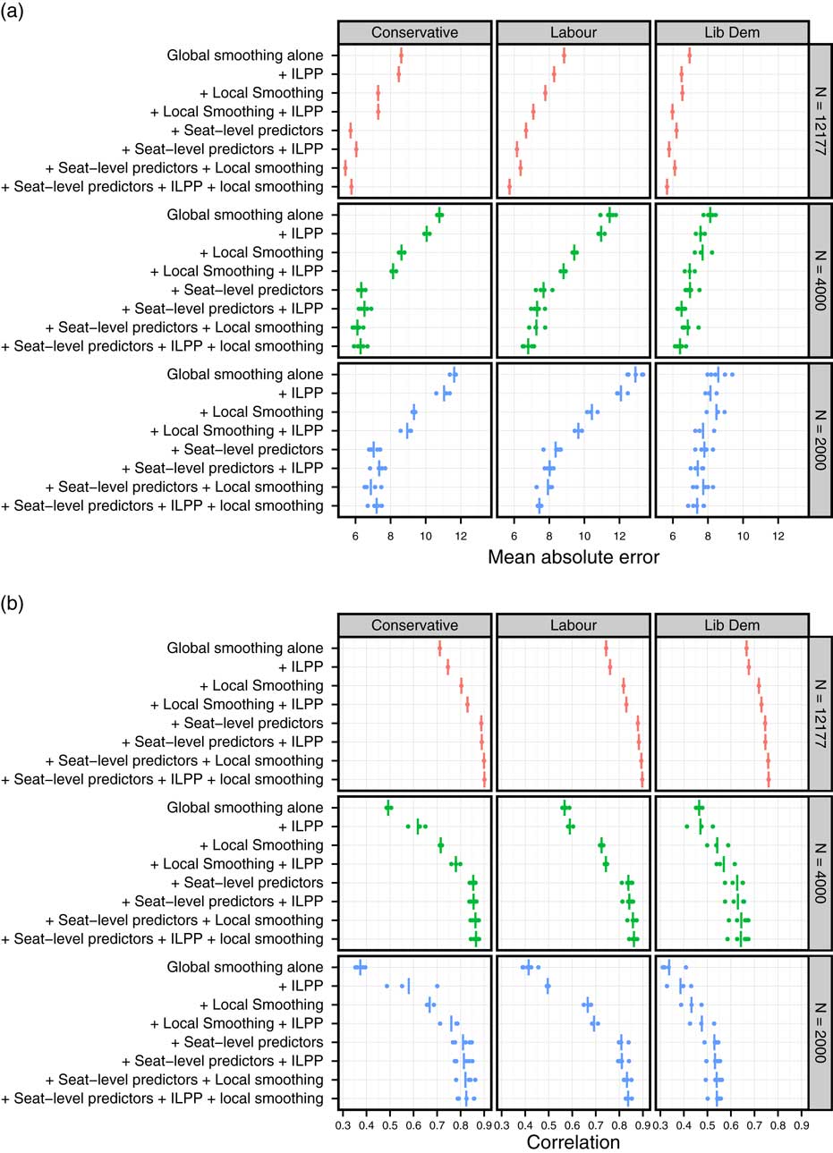
Fig. 2 External validation: performance across sample sizes Note: ILPP=individual-level predictors and post-stratification.
Based on Figure 2, the relative contributions from each source of information appear to follow a similar order whether working with the full sample (N=12,177) or the two smaller survey samples. For all parties and all sample sizes, the performance of constituency estimates is substantially improved by the introduction of constituency-level predictors. The gains from local smoothing and ILPP are larger in smaller samples; however, they remain modest relative to those from constituency-level predictors, particularly once constituency-level predictors are already included in the estimation strategy.
How good are our best estimates?
Researchers considering using constituency opinion estimates in applied work need to know not just how each information source contributes to the quality of estimates, but also how good these estimates are in absolute terms (Buttice and Highton Reference Buttice and Highton2013, 453). One way to put the performance of our best-performing models in context is to take the RMSE of these estimates and roughly approximate the necessary constituency sample size one would need to ensure an equivalent RMSE if using direct estimation.Footnote 14 We begin by considering the RMSE for sample sizes of 2000, as this sample size is feasible for researchers acting outside of national election studies. The RMSE of our best-performing estimates, which were generated from average constituency sample sizes of just over three respondents, varies between 8.9 and 9.6 across sub-samples. To achieve equivalent RMSEs from direct estimation, one would need constituency sample sizes of between 23 and 26, corresponding to national samples of between 14,000 and 16,000. In other words, in this instance, incorporating extra information to generate constituency opinion estimates increases effective sample size by a factor of at least 7. If instead we consider the RMSE for our largest sample size of 12,177, we would need constituency sample sizes of 36–41, corresponding to national samples of between 23,000 and 26,000, or a (much more expensive) doubling of the sample.
This assumes that this hypothetical national survey has exactly zero bias, which is unrealistic. To incorporate realistic levels of bias in the benchmark, we could instead compare the MAEs from the better-performing models with those generated when large constituency-specific surveys are run in the lead-up to by-elections. We were able to collect information on 13 such pre-by-election polls. The average sample size of these polls is 855, with a minimum of 500 and maximum of 1503. Taking actual by-election results as measures of true opinion, the MAEs of the vote share estimates from the 13 by-election surveys were 5.03, 3.32, and 2.71 for the Conservatives, Labour, and Liberal Democrats, respectively. The MAEs of our best-performing 2010 vote share estimates, using the full sample, lie between 5.67 and 5.77. Thus, despite a huge disadvantage in terms of sample size, the MAEs of our best-performing estimates are close to those of by-election polls.
New Cross-Validation Evidence
Cross-Validation Strategy
So far, we have tested strategies for estimating constituency opinion through external validation of vote share estimates. However, applied researchers are likely to want estimates of constituency-level opinion on specific policy issues, not just party support. Therefore, it is important to ask whether the relative contribution of different information sources is likely to change drastically when estimating constituency opinion on specific policy issues. It is difficult to use external validation to address this question because we very rarely observe true values of constituency-level opinion on specific policy issues. Instead, we employ a cross-validation approach, as used by Lax and Phillips (Reference Lax and Phillips2009), Warshaw and Rodden (Reference Warshaw and Rodden2012), and Buttice and Highton (Reference Buttice and Highton2013) in the US context.
To perform our cross-validation, we use the BES Cumulative Continuous Monitoring (CMS) Survey data, which combines responses to over 90 monthly internet surveys fielded by YouGov between 2004 and 2012.Footnote 15 Our opinion variable is disapproval of British membership of the European Union, originally measured on a four-point scale but re-coded into a binary variable equaling 1 if the respondent disapproves of Britain’s EU membership, and 0 otherwise. We have 57,440 non-missing observations from respondents whose constituency location is known.
We randomly split our 57,440 respondents into estimation and holdout samples. We then ran each of the nine estimation strategies used in the external validation study and compared our EU disapproval estimates with “true” values defined by the disaggregated holdout sample. To assess whether the contribution of different information types varies with the size of the estimation sample, we performed the cross-validation for three sizes of estimation sample: 2000, 4000, and 10,000. To account for sampling error, we ran five simulations for each estimation sample size.
We make three changes to the estimation strategies used in the external validation study. First, we add 2010 constituency vote shares for the three main parties as constituency-level predictors; in contrast to our external validation study, these are not lagged versions of the quantity of interest, but instead represent auxiliary political information that researchers are likely to have access to. Second, we drop two individual-level predictors used in the external validation study but not measured in the CMS data (sector of employment and level of education). Third, the post-stratification weights we use for ILPP are based on the observed joint distribution of demographic characteristics among respondents from each constituency in the full survey data (rather than the joint distribution in the real constituency population, based on census data). We do this because in the cross-validation setup our populations of interest are no longer the real constituency populations but constituency sub-samples of the holdout data. Note that defining post-stratification weights in this way also means that we can assess the contribution of ILPP in the “ideal” scenario where post-stratification weights are highly accurate.
Results
Figure 3 presents the results of our cross-validation study, arrayed by estimation strategy (columns) and size of estimation sample (rows). For a given estimation strategy-sample size combination we have several sets of estimates (one for each random split of the data into “estimation sample” and “holdout sample”), so for each such combination we plot the set of estimates with the median MAE score and print the average MAE, correlation, and RMSE.
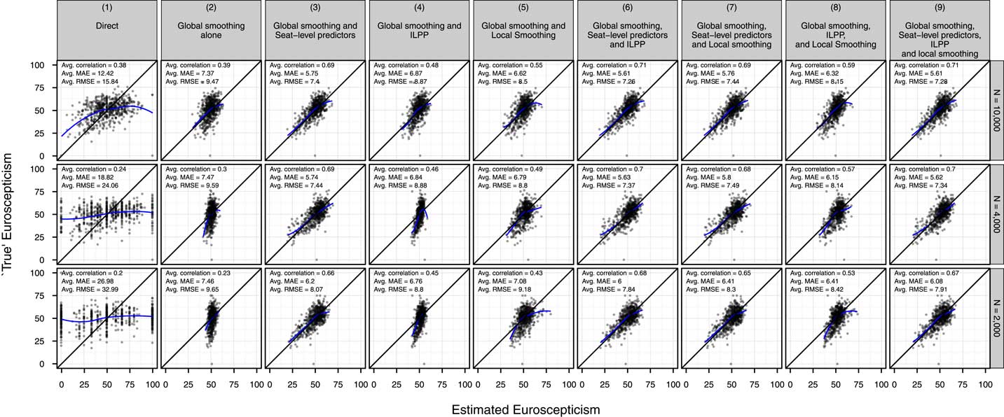
Fig. 3 Cross-validation: estimated constituency EU disapproval versus “true scores” Note: ILPP=individual-level predictors and post-stratification; MAE=mean absolute error; RMSE=root mean square error.
Figure 3 suggests that when we estimate constituency opinion on a specific issue, the relative gains from using different information sources are broadly similar to those found when estimating constituency vote shares.
First, relying exclusively on information from constituency sub-samples with direct estimation (column 1) again leads to very poor estimates, with high MAEs and very low correlations.
Second, introducing global smoothing (column 2) reduces MAEs somewhat but does little to improve correlations because estimates are simply shrunk toward the sample mean.
Third, as with the external validation, the introduction of constituency-level predictors leads to substantial improvements in both MAEs and correlations. When constituency-level predictors are added to a simple model using only global smoothing (column 3 versus 2), correlations jump by >0.3 and MAEs improve by >1 percentage point. When constituency-level predictors are added to more complex models, which already include either ILPP, local smoothing, or both (column 6 versus 4, 7 versus 5, and 9 versus 8, respectively), correlations increase by at least 0.1 and MAEs improve by at least 0.3.
Fourth, the relative contribution of ILPP here appears to be greater than in the external validation study. Recall that this is a favorable situation for ILPP, as the post-stratification weights used are unusually accurate. When ILPP is added to any estimation strategy (column 4 versus 2, 6 versus 3, 8 versus 5, or 9 versus 7), correlations on average increase by >0.05 while MAEs improve by at least 0.15 and usually more.
Fifth, the inclusion of constituency-level predictors appears to explain away a lot of the spatial dependencies that local smoothing exploits. When constituency-level predictors are not in use, adding local smoothing leads to jumps in correlations of between 0.05 and 0.2 and MAE reductions of between 0.4 and 0.65 (comparing column 5 versus 2 and 8 versus 4). However, when constituency-level predictors are already in use, the corresponding gains are much smaller: below 0.01 for correlations, and between 0.01 and 0.2 for MAEs.
In sum, this cross-validation evidence again suggests that researchers can expect to improve constituency opinion estimates primarily through the careful selection of constituency-level predictors. Nevertheless, the best estimation strategy for all sample sizes utilizes all possible sources of information. Thus, while our results consistently suggest that constituency-level predictors provide by far the most predictive power given the costs of collection, implementation, and estimation, it is nonetheless true that more information is better. If researchers can afford to incorporate all sources of information, they will get better estimates.
MAEs are higher and correlations are lower in this cross-validation study than in the external validation study. But, even for the largest estimation sample of 10,000, the use of extra information sources to estimate constituency opinion still increases effective sample size by a factor of 2.5: using direct estimation one would need an average constituency sample size of 39 (corresponding to a national sample size of around 25,000) to achieve the average RMSE of the best-performing constituency Euroscepticism estimates we generate based on average constituency sample sizes of 16. With the smallest sample size, correlation, MAE, and RMSE are all nearly as good, and so the effective increase in sample size is nearly ten times as large. With average correlations of around 0.7 and MAEs around 5.5 percent—which corresponds to just over half a SD of “true” constituency Euroscepticism—the estimates for all of the sample sizes are similarly usable.
Conclusion
In this paper, we have discussed methods for improving constituency-level political opinion estimates by supplementing national survey data with a number of different types of auxiliary information. To assess the improvements yielded by these different types of information, we conducted an external validation study and a cross-validation study in the British context where constituencies are (relatively) numerous and (relatively) small. These are the first results simultaneously comparing the relative contributions of all four possible sources of information used in MRP—global smoothing, ILPP, constituency-level predictors, and local smoothing. In both studies, we found that the best-performing estimates came from including all sources of information. However, we found that most of the gains over direct estimation came from including a suite of constituency-level predictors.
This finding—which is consistent with previous studies conducted in the United States—is good for researchers, as constituency-level predictors are the easiest (and sometimes the only possible) option for researchers to employ in many settings. There are gains to be had from including individual-level predictors and post-stratification or local smoothing, and we were able to suggest circumstances in which each of these might be particularly useful (sample unrepresentativeness in the case of ILPP; limitations of constituency-level predictors in the case of local smoothing), but these two options have more stringent data availability requirements and increase computational burden substantially.
In general, it is hard to validate methods like those considered in this paper. In a narrow sense, our results only apply when estimating opinion for (a) UK (b) parliamentary constituencies, when (c) predicting vote share and Euroscepticism using (d) particular sets of constituency and demographic variables. Yet, given the overlap between some of our findings (particularly those with respect to constituency-level predictors) and some of the findings from the much more extensive literature on the estimation of state- and district-level opinion in the United States, our results broaden the evidence base for certain recommendations to scholars looking to apply these techniques to estimate opinion in different settings.
First, in situations like the United Kingdom, characterized by a large number of areal units, effort should be focused on the search for area-level predictors thought to be highly correlated with the opinion of interest. The number of area-level predictors for inclusion in a model may be limited in practice by the number of areal units: in particular, the greater the ratio of area-level predictors to areal units, the greater the risk of over-fitting (Lax and Phillips Reference Lax and Phillips2013).
Second, interpreting our findings in the light of other research, the more limited the number of areal units, the more quickly researchers will wish to move on to ILPP, which has been found to work particularly well in the Swiss case, where the number of areal units is 28 (Leemannn and Wasserfallen Reference Leemannn and Wasserfallen2014).
Third, it remains the case that local smoothing has in our tests always improved the quality of estimates, and so researchers who wish to maximize the quality of their estimates, regardless of the cost, should use local smoothing. Incurring the (computational and data) costs of local smoothing becomes more important if the search for area-level predictors is severely limited. Unscheduled electoral redistricting, for example, may mean that no information has been collected at the relevant level.Footnote 16 In such cases the use of ILPP is also likely to be precluded, meaning that local smoothing is the only remaining feasible option (Selb and Munzert Reference Selb and Munzert2011).
Fourth, if neither ILPP nor local smoothing is possible, then usable estimates of local opinion are possible as long as there are good area-level predictors available, the number of areal units is sufficiently large (where by sufficiently large we mean large enough for a linear regression of the opinion on the area-level predictors), and where either the sample size is as large as our full sample (12,177), or the number of respondents per areal unit is as large as it is in our full sample (19.3).
The dominant performance of constituency-level variables in these models is perhaps not surprising, because such variables offer the most direct information about the estimand, which is also at the constituency level. Where a high partial correlation is sufficient for a constituency-level variable to improve prediction, for an individual-level variable to improve prediction it must both be highly correlated with opinion, and also highly varying in prevalence across constituencies. By a similar logic, the major sources of geographic variation in opinion can often be captured by constituency-level covariates, especially measures of region or population density.
Our work invites further research applying these constituency opinion estimates, or using the strategies described herein to generate new estimates, to substantive questions about representation. While advances in the estimation of public opinion at the constituency-level in the United States have revitalized a previous literature on dyadic representation (Miller and Stokes Reference Miller and Stokes1963; Erikson, Wright and McIver Reference Erikson, Wright and McIver1993; Hill and Hurley Reference Hill and Hurley1999), that literature—with isolated exceptions (Converse and Pierce Reference Converse and Pierce1986)—never gained traction in Europe (Powell Reference Powell2004), due in part to greater party discipline but due also to the lack of measures of opinion. The strategies discussed here can provide researchers outside of the United States with an intuition concerning the relative performance of strategies which will help them to proceed to dealing with substantive questions.


 Open access